Gauss’ and Stokes’ Theorems#
About the project#
Duration: 15–40 hours (including typesetting final report in LaTeX)
Prerequisites: Multivariable calculus (grad/div/curl), line & surface integrals, vector fields, basic linear algebra, basic physics (charge/current/fields), basic Python (optional)
Python packages: NumPy, sympy, matplotlib (optional)
Learning objectives: Use Gauss’ and Stokes’ theorems to relate integral and differential forms, derive the continuity equation, analyze inconsistencies in the pre-Maxwell equations, understand Maxwell’s displacement current and electromagnetic wave equations
In this assignment we study vector analysis with applications in electromagnetism. Without explanation we postulate the governing equations of electromagnetism for the electric field \(E\) (force per charge) and the magnetic field \(B\) (force per charge per velocity), and then use vector analysis to illuminate various mathematical relations.
1 Mathematical notation#
We use the following mathematical notation in this assignment. The unit vectors in the three Cartesian coordinate directions are called \(e_x\), \(e_y\) and \(e_z\). The partial derivatives with respect to the time and space coordinates are denoted with a compact notation as
Here we have introduced the vector operator “\(\nabla\)”, called “nabla” (after Ancient Greek “harp”, since the symbol resembles a small harp), which turns out to be very practical. We can see that nabla has three components just like an ordinary vector, \(a=e_x a_x + e_y a_y + e_z a_z\), and nabla even has more similarities with vectors, as we will see during this assignment.
The first-order Taylor expansion of a scalar function \(f(x)\) of one variable around the point \(x_0\) to first order in the small change \(\Delta x\) is
The first-order Taylor expansion of a scalar function \(f(r)=f(x,y,z)\) of three variables around the point \(r_0=e_x x_0 + e_y y_0 + e_z z_0\) to first order in the small change \(\Delta r=e_x\Delta x + e_y\Delta y + e_z\Delta z\) naturally contains three contributions to the increment of \(f(r_0)\), one for each variable corresponding to the single increment \(\Delta x\,\partial_x f(x_0)\) to \(f(x_0)\) in Eq. (2),
Here the compact dot-product notation \(\Delta x\,\partial_x + \Delta y\,\partial_y + \Delta z\,\partial_z = \Delta r\cdot\nabla\) known from ordinary vectors, \(a_x b_x + a_y b_y + a_z b_z = a\cdot b\), has been used in the last line. Notice how compact, yet still unambiguous, the notation becomes by using the nabla operator “\(\nabla\)”.
For a vector function \(V(r)=e_x V_x(x,y,z)+e_y V_y(x,y,z)+e_z V_z(x,y,z)\) of three variables, we gain even more from the compact notation. The Taylor expansion of \(V(r)\) around the point \(r_0\) to first order in the small change \(\Delta r=e_x\Delta x+e_y\Delta y+e_z\Delta z\) is performed componentwise corresponding to Eq. (3), and we get
Note the structural similarity between Eq. (2) and Eq. (4c), while a concrete calculation of the latter still requires use of the extensive expressions in Eq. (2) and Eq. (4a).
Analogous to the dot product \(a\cdot b\) and the cross product \(a\times b\), we naturally (yes, wait and see) introduce the so-called divergence \(\nabla\cdot V\) and curl \(\nabla\times V\) of a vector field \(V(r)\) as
Consider a curve \(C(p)\) in space with line element \(dr\), parameterization \(r=r(p)\), Jacobian \(|\partial_p r|\), and the tangent vector \(t=\partial_p r/|\partial_p r|\), where \(p\in[a,b]\subset\mathbb{R}\) is a 1D parameter interval. The line integral over \(C\) for respectively a scalar field \(f(r)\) and a vector field \(v(r)\) is then defined as
Consider a surface \(S(p,q)\) in space with area element \(da\), parameterization \(r=r(p,q)\), Jacobian \(|\partial_p r\times \partial_q r|\), and normal vector \(n=(\partial_p r\times\partial_q r)/|\partial_p r\times \partial_q r|\), where \(\{p,q\}\in P\subset\mathbb{R}^2\) is a 2D parameter domain. The surface integral over \(S\) for respectively a scalar field \(f(r)\) and a vector field \(v(r)\) is defined as
Consider a volume \(V(s,p,q)\) in space with volume element \(d\tau\), parameterization \(r=r(s,p,q)\) and Jacobian \(\big|\partial_s r\cdot(\partial_p r\times \partial_q r)\big|\), where \(\{s,p,q\}\in Q\subset\mathbb{R}^3\) is a 3D parameter domain. The volume integral over \(V\) for respectively a scalar field \(f(r)\) and a vector field \(v(r)\) is defined as
2 Introduction: basic electromagnetic concepts and fields#
Consider an electric point charge \(q\) (for example an electron) which at a given time \(t\) moves with velocity \(v_q\) as it passes through the point \(r\). The total electromagnetic force \(F_q\) on the particle is then given by the sum of the electric force \(F_q^{\mathrm{elec}}\) and the magnetic force \(F_q^{\mathrm{magn}}\),
This force law defines the two basic vector fields in electromagnetism, the electric field \(E(r,t)\) (force per charge) and the magnetic field \(B(r,t)\) (force per charge per velocity). These two vector fields are assumed to be differentiable at every point \(r\) in space and at all times \(t\).
A central theorem in vector analysis, Helmholtz’ theorem, says that a given suitably differentiable vector field \(V\) is fully determined if its divergence \(\nabla\cdot V\) and its curl \(\nabla\times V\) are known. A consequence is that there are four governing equations in electromagnetism, namely equations for \(\nabla\cdot E\), \(\nabla\cdot B\), \(\nabla\times E\) and \(\nabla\times B\).
Over approximately the 120 years from the 1740s until 1860, most of the laws of electromagnetism were found, which can be summarized as follows. There are two types of charges called positive and negative. Charge is conserved, in that it can neither be created nor destroyed, but only moved around. One can think of charge as discrete point charges or as a continuous charge density \(\rho(r,t)\) (charge per volume), which can vary in space and time. Around any charge there is an electric field (Coulomb’s and Gauss’ laws), and the total electric field \(E(r,t)\) at the point \(r\) at time \(t\) is given as the sum of these elementary electric fields (the superposition principle). There are no magnetic monopoles (“charges”) that create magnetic fields; instead, an electric current density \(J(r,t)\) (charge per area per time) creates a magnetic field \(B(r,t)\) (Ørsted’s and Ampère’s laws). Finally, it turns out that electric fields are not only created by local charge densities, but also by time-varying magnetic fields (Faraday’s law of induction). Around 1860, one believed that the four governing equations in electromagnetism had the following form, which we may call the pre-Maxwell equations,
It is the mathematical structure of this system of equations that we will study in this assignment. In particular, we will modify Ampère’s law (10-iv), a modification which Maxwell discovered in the years 1861–65 was necessary, and which led to the final, currently used formulation of electromagnetism’s four Maxwell equations. Maxwell’s modification not only clarified inconsistencies in the electromagnetism theory of the time, but also led to Maxwell predicting the existence of electromagnetic waves (which were first demonstrated experimentally 26 years later), and that all electrical, magnetic and optical phenomena could be explained with one unified theory, Maxwell’s electromagnetic theory. And not only that: only 40 years after Maxwell’s theory was launched, it formed the basis for Einstein’s special theory of relativity.
3 Gauss’ theorem (the divergence theorem)#
Gauss’ theorem (Joseph-Louis Lagrange [1773] and Carl Friedrich Gauss [1835]), also called the divergence theorem, is a central theorem in vector analysis. For a given region \(\Omega\) in space it relates the flux integral of a vector field over the surface \(\partial\Omega\) with outward surface normal \(n\) to the divergence of the field throughout \(\Omega\). For a suitably differentiable vector field \(J(r)\) defined in all of space, the following holds for an arbitrary subregion \(\Omega\) of space,
In the following we prove this theorem using the (infinitesimally) small rectangular box \(\Delta\Omega\) shown in Figure 1 with side lengths \(\Delta x\), \(\Delta y\) and \(\Delta z\), volume \(\Delta\tau=\Delta x\Delta y\Delta z\) and the six surface areas \(\Delta a_i\) each with its outward-pointing normal vector \(n_i\): \(n_1\Delta a_1=-e_x\Delta y \Delta z\), \(n_2\Delta a_2=+e_x\Delta y\Delta z\), …, and \(n_6\Delta a_6=+e_z\Delta x\Delta y\).
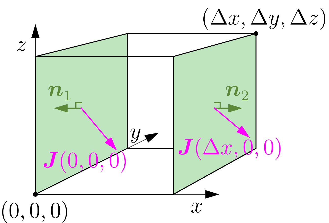
Figure 1: The Gauss box \(\Delta\Omega\).
Exercise 1
Express the flux integral \(\Phi(J,\Delta\Omega)=\oint_{\partial(\Delta\Omega)} J\cdot n\,da = \sum_{i=1}^{6}\int_{\Delta a_i} J(r_i)\cdot n_i\,da_i\) as a sum of six contributions, one from each face, and then combine the three pairs of opposite surface integrals, where the integrand is respectively \(J_x(r)\), \(J_y(r)\), \(J_z(r)\).
Exercise 2
Prove Gauss’ theorem for \(\Delta\Omega\) by Taylor-expanding the integrands in the surface integrals above to lowest order in \(\Delta x\), \(\Delta y\) and \(\Delta z\), e.g.
\(J_x(\Delta x,y,z)\approx J_x(0,y,z)+\partial_x J_x(0,y,z)\,\Delta x\)
and similarly for \(J_y(x,\Delta y,z)\) and \(J_z(x,y,\Delta z)\).
Exercise 3
Show Gauss’ theorem for an arbitrary region \(\Omega\) by dividing it into a very large number of infinitesimally small boxes, each as in Figure 1, and argue for the pairwise cancellation of \(J\cdot n\) on all internal boundary surfaces between neighboring boxes.
Hint: Use the Riemann integral concept.
The concept of divergence \(\nabla\cdot J\) of a vector field \(J\) was introduced because of its role in Gauss’ theorem. As an alternative to the definition (11d) in explicit Cartesian coordinates, one can define the divergence \(\nabla\cdot J\) in the following coordinate-free form, as a limit of the flux integral per volume,
4 Stokes’ theorem (the curl theorem)#
Stokes’ theorem [George Green, William Thompson (Lord Kelvin), George G. Stokes (1828–1850)], also called the curl theorem, is another central theorem in vector analysis. For a given surface \(S\) in space bounded by the boundary curve \(\partial S\), it relates the circulation integral of a vector field along the boundary curve \(\partial S\) to the curl of the field over the whole surface \(S\). For a suitably differentiable vector field \(B(r)\) defined in all of space, the following holds for an arbitrary surface \(S\) in space, see Figure 2,
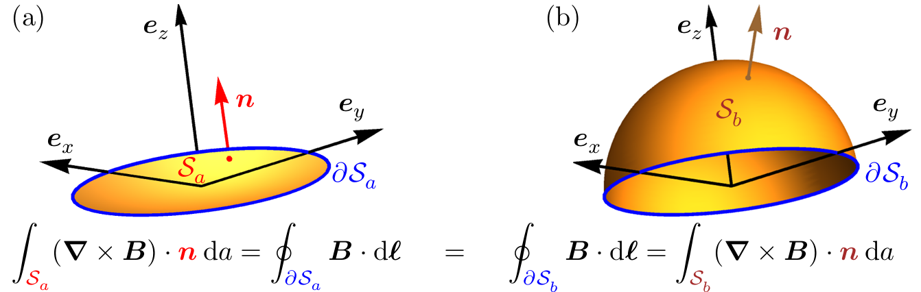
Figure 2: Two surfaces \(S_a\) and \(S_b\) in space bounded by the same boundary, \(\partial S_a = \partial S_b\) (blue curve). In the concrete example the boundary curve is a circle of radius \(R\), \(S_a\) is a circular surface in the \(xy\)-plane with radius \(R\), and \(S_b\) is the hemisphere surface with radius \(R\) in the positive half-space \(z\ge 0\). Since \(S_a\) and \(S_b\) are bounded by the same boundary, Stokes’ theorem implies that the flux integrals over the two surfaces of the curl \(\nabla\times B\) of an arbitrary vector field \(B\) are identical, \(\Phi(\nabla\times B,S_a)=\Phi(\nabla\times B,S_b)\).
In the following we prove this theorem using the (infinitesimally) small surface, the right triangle \(\Delta S\) in the \(xy\)-plane shown in Figure 3, formed by the corner points \(A(0,0,0)\), \(B(\Delta x,0,0)\), and \(C(\Delta x,\Delta y,0)\). \(\Delta S\) has angles \(\angle A=\alpha\), \(\angle B=\pi/2\) and \(\angle C=\pi/2-\alpha\) and area \(\Delta a=\tfrac{1}{2}\Delta x\Delta y\). The side lengths in triangle \(ABC\) are the hypotenuse \(|AC|=\Delta L\) and the legs \(|AB|=\Delta x=\Delta L\cos\alpha\) and \(|BC|=\Delta y=\Delta L\sin\alpha\). Based on the definition (6b) we choose parameterizations of the three sides as respectively \(r_{AB}(p)=p\,e_x\) with \(p\) from \(0\) to \(\Delta x\), \(r_{BC}(p)=\Delta x\,e_x + p\,e_y\) with \(p\) from \(0\) to \(\Delta y\), and \(r_{CA}(p)=p\cos\alpha\,e_x + p\sin\alpha\,e_y\) with \(p\) from \(\Delta L\) to \(0\). The sides’ tangent vectors are called \(t\).
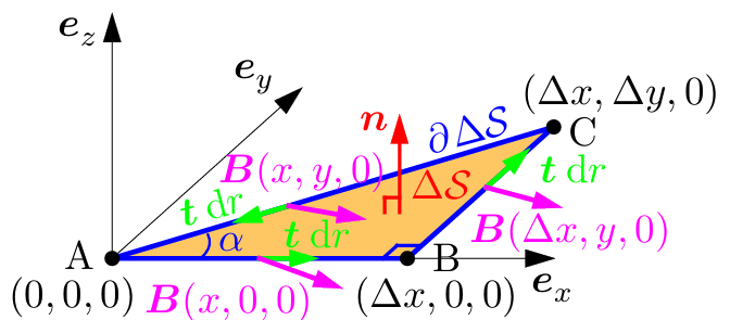
Figure 3: The Stokes surface \(\Delta S\), triangle \(ABC\).
Exercise 4
Split the circulation integral of \(B\) along the boundary \(\partial\Delta S\) into three contributions\[\begin{equation*} \oint_{\partial\Delta S} B\cdot t\,dr = \int_0^{\Delta x} B(r_{AB}(p))\cdot\partial_p r_{AB}(p)\,dp + \int_0^{\Delta y} B(r_{BC}(p))\cdot\partial_p r_{BC}(p)\,dp + \int_{\Delta L}^{0} B(r_{CA}(p))\cdot\partial_p r_{CA}(p)\,dp, \end{equation*}\]and show that in the limit \(\Delta L\to 0\) one gets
\[\begin{equation*} \oint_{\partial\Delta S} B(r)\cdot t\,dr \approx \big(\partial_x B_y(0)-\partial_y B_x(0)\big)\,\Delta a. \end{equation*}\]Hint: In the integrands use the Taylor expansion \(B(r)\approx B(0)+(r\cdot\nabla)B(0)\) valid for \(0\le r\le \Delta L\), neglecting terms of order \((\Delta L)^2\) and higher.
Exercise 5
Show Stokes’ theorem for an arbitrary curved surface \(S\) bounded by the closed curve \(\partial S\), by first choosing a large number of closely spaced points distributed on the surface and its boundary \(\partial S\). Let nearest-neighbor points form the corners of many small triangles that together form a faceted surface approximately equal to \(S\). Consider how non-right triangles can be split into two right triangles, so that the final faceted surface consists of \(N\) right triangles \(\Delta S_i\), each with its boundary \(\partial\Delta S_i\) and its local coordinate system corresponding to Figure 3. Briefly account for the pairwise cancellation of line integrals along all internal boundary lines between neighboring triangles, even if these do not lie in the same plane.
Hint: Use the Riemann integral concept.
The concept of curl \(\nabla\times B\) of a vector field \(B\) was introduced because of its role in Stokes’ theorem. As an alternative to the definition (13b) in explicit Cartesian coordinates, one can define the curl \(\nabla\times B\) in coordinate-free form, as a limit of the circulation integral per area,
5 Integral statements: Coulomb’s and Ørsted–Ampère’s laws#
In 1785, Charles-Augustin de Coulomb published his famous law for the electrostatic force between two charges: the force acts in a direction parallel to the line connecting the two charges, and it is proportional to the inverse of the square of the distance between the charges. Consider a point source charge \(Q\) placed at the origin \(0\), and a test charge \(q\) at an arbitrary point \(r\). Then the force on \(q\) at \(r\) from \(Q\) at \(0\) can be written as
We now show, using the divergence theorem, that this law is contained in Gauss’ law (10-i).
Exercise 6
From Gauss’ law (10-i) to Coulomb’s law. Express the force from \(Q\) on \(q\) as \(F_{q\leftarrow Q}(r)=qE_Q(r)\), and determine the electric field \(E_Q(r)\) from the point charge \(Q\) at the origin using a test volume \(\Omega\) in the form of a sphere \(K_r\) with radius \(r\) and center at the origin.
Hint: Integrate Eq. (10-i) over \(\Omega=K_r\), use the divergence theorem, and use the following three facts: (1) the total charge contained in \(K_r\) is \(Q\) for all values of \(r\), (2) the spherical symmetry of the point charge \(Q\) implies that the electric field only has a radial component, \(E_Q(r)=E_r(r)e_r\), and (3) for the surface normal on \(\partial K_r\) we have \(n=e_r\).
The similarity between Coulomb’s force law (15) from 1785 and Newton’s law of universal gravitation between two point masses \(m\) at \(r\) and \(M\) at \(0\), \(F_{m\leftarrow M}(r)=G\frac{mM}{r^2}e_r\), published almost a hundred years earlier in 1687, gave natural philosophers of the time a strong belief that all laws of nature could be reduced to such inverse-square laws along the line connecting particles. Furthermore, one believed that electric and magnetic phenomena were completely independent of each other.
It was therefore a radically groundbreaking discovery that Hans Christian Ørsted made in 1820, when he first demonstrated that an electric current generates a magnetic field, and then that this magnetic field influences a magnetic needle with a force perpendicular to the current direction. Within a short time the skepticism of especially French physicists was transformed into a solid mathematical theory developed primarily by André-Marie Ampère, Jean Baptiste Biot and Felix Savart.
If an electric current \(I\) (charge per time) is sent through a (infinitely) long cylindrical wire with radius \(a\) placed along the \(z\)-axis, a magnetic field \(B\) will arise around the wire. Using cylindrical coordinates \(r=(s,\phi,z)\), where \(s\) is the perpendicular distance to the \(z\)-axis and \(\phi\) the usual azimuthal angle, the resulting magnetic field \(B(r)\) at an observation point \(r\) outside the wire can be written as
Exercise 7
Symmetry analysis. Assume that the current \(I\) in the long thin wire is formed by a rotationally symmetric current density independent of the \(z\)-coordinate, \(J(r)=J_z(s)e_z\). First argue that the symmetry of the system implies that the magnetic field can only depend on the radial coordinate \(s\), \(B(r)=B(s)\). Then show that \(B_s(s)=0\) by considering \(B\) around the wire after performing the following two transformations, which bring the system back to its starting point: (1) reverse the current direction in the wire, whereby \(B(s)\) changes sign, (2) rotate the wire \(180^\circ\) around the \(x\)-axis. Finally show that Ampère’s law (10-iv) with \(J(r)=J_z(s)e_z\) implies that \(B_z(s)\) is constant, and in fact \(0\) since \(B\) tends to zero far from the wire. Thus it is shown that the final form of the magnetic field is \(B(r)=B_\phi(s)e_\phi\).
Exercise 8
Show Eq. (16) by combining Ampère’s law (10-iv), where by symmetry \(B(r)=B_\phi(s)e_\phi\) and \(J(r)=J_z(s)e_z\) as shown above, with Stokes’ theorem (13a) for a circle \(\partial S\) in the \(xy\)-plane with center on the \(z\)-axis and radius \(s\).
Hint: The circulation integral of \(B\) can be carried out explicitly, and the current \(I\) (charge per time) can be written as a surface integral perpendicular to the wire of the current density \(J\) (charge per area per time).
6 Charge conservation and the continuity equation#
In continuum physics, Gauss’ theorem is used together with the conservation laws of physics to derive the governing partial differential equations for the relevant fields. As an example we derive the so-called continuity equation, which expresses charge conservation.
Exercise 9
Derivation of the continuity equation. Consider an arbitrary but fixed subregion \(\Omega\) in space with surface \(\partial\Omega\). Electric charge can freely cross the surface, so the total charge \(Q(t)\) in \(\Omega\) depends on time. We are interested in studying the rate \(\partial_t Q(t)\) at which the charge inside \(\Omega\) changes, expressed by the charge density \(\rho(r,t)\) (charge per volume) and the charge current density \(J(r,t)\) (charge per area per time). Conservation of charge means that the total charge in \(\Omega\) can only change by charge flowing through the surface \(\partial\Omega\). Charge can therefore not (in classical physics) suddenly appear at a point in space. Argue that the rate of change \(\partial_t Q\) of charge can be expressed both as the volume integral \(\partial_t Q = V(\partial_t \rho,\Omega)\) and as the flux integral \(\partial_t Q = \Phi(-J\cdot n,\partial\Omega)\). Rewrite the flux integral as a volume integral using Gauss’ theorem, and then argue that since the resulting identity between the two volume integrals holds regardless of the choice of \(\Omega\), the two integrands must be identical, and the continuity equation is thereby shown,\[\begin{equation*} \partial_t \rho = -\nabla\cdot J,\ \text{the continuity equation expressing charge conservation}.\tag{17} \end{equation*}\]
7 Fundamental inconsistencies in the pre-Maxwell equations#
For about 10 years (1855–1865), James Clerk Maxwell studied the theoretical foundations of electromagnetism. He discovered and corrected fundamental inconsistencies in the pre-Maxwell equations and thereby developed the modern electromagnetic theory, also called Maxwell’s theory. We will look at two such inconsistencies in Eq. (10).
Exercise 10
Lack of charge conservation in Eq. (10). Combine Eq. (11d) and Eq. (13b) and show that for an arbitrary differentiable vector field \(B\) one has \(\nabla\cdot(\nabla\times B)=0\), and that Eq. (10-iv) therefore gives \(\nabla\cdot J=0\) for all magnetic fields \(B(r,t)\), in contradiction with charge conservation expressed by the continuity equation (17).
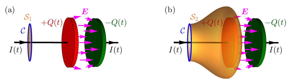
Figure 4: Charging of a capacitor with a time-dependent electric current \(I(t)\) (black wire). The capacitor’s one metal plate (red) has a time-dependent positive charge \(+Q(t)\), while the other (green) has a corresponding negative charge \(-Q(t)\). The system is analyzed with a circulation integral of \(B(r,t)\) along the circle \(C\) (blue) centered on the wire in a plane perpendicular to it. \(C\) is the boundary for both the plane circular surface \(S_1\) (a) and for the curved pear-shaped surface \(S_2\) (b). \(I(t)\) passes through \(S_1\) but not \(S_2\), which instead encloses both wire and the positive capacitor plate. There is an electric field \(E(r,t)\) (magenta) in the capacitor gap and near its edge, while \(E(r,t)\) is zero everywhere else in the system.
Exercise 11
Electric current or not during charging of a capacitor? A capacitor consists of two metal plates that are placed close to each other, but without electrical contact, see Figure 4. A capacitor can be charged with electric charge by connecting it to a battery (preferably in series with a resistor), such that an electric current \(I(t)=\Phi(J,S)\) flows into the one plate, which therefore obtains a growing positive charge \(Q(t)\), while a corresponding electric current flows away from the other plate, which therefore obtains a negative charge \(-Q(t)\). The capacitor therefore always has total charge zero, but there is an electric field \(E(r,t)\) in and slightly outside the gap between the plates, which points (roughly) in the direction from the positive to the negative plate. Now use Stokes’ theorem on Ampère’s law (10-iv) with the two different surfaces shown in Figure 4: \(S_1\) (a plane circular surface) and \(S_2\) (a curved pear-shaped surface), which have the circle \(C=\partial S_1=\partial S_2\) as common boundary. Show that with \(S_1\) we obtain as expected a current \(I(t)\neq 0\), while \(S_2\) very surprisingly gives the obviously wrong answer \(I(t)=0\).
8 Maxwell’s equations#
In the years 1861–65, James Clerk Maxwell published five articles in which he developed the full classical electromagnetic theory, which (with Oliver Heaviside’s elegant vector formulation from 1884) in only four equations summarizes all electromagnetic phenomena, except the atomic processes of absorption and emission of electromagnetic radiation, with \(\epsilon_0 = 8.854\times 10^{-12}\ \mathrm{F/m}\) and \(\mu_0 = 1.257\times 10^{-6}\ \mathrm{H/m}\),
This final formulation of electromagnetic theory differs from the pre-Maxwell theory (10) by the presence of the so-called Maxwell displacement current density \(\epsilon_0\partial_t E\), which multiplied by the constant \(\mu_0\) has been added to the right-hand side of Ampère–Maxwell’s law (18-iv). We now verify that the two examples of fundamental inconsistencies studied in Exercises 10 and 11 have been repaired.
Exercise 12
Charge conservation in Maxwell’s equations. Repeat the considerations in Exercise 10, but now where \(J\) is replaced by \(J+\epsilon_0\partial_t E\).
Hint: A new term \(\nabla\cdot(\epsilon_0\partial_t E)\) appears, which can be reduced using Gauss’ law (18-i), whereby the continuity equation (17) emerges. Charge conservation is thus contained implicitly in Maxwell’s equations.
Exercise 13
Maxwell’s analysis of the capacitor charging. Repeat the considerations in Exercise 11, but now where \(J\) is replaced by \(J+\epsilon_0\partial_t E\).
Hint: Argue that the new flux term \(\Phi(\epsilon_0\partial_t E,S_2)\) is identical to \(\Phi(\epsilon_0\partial_t E,S_1+S_2)\), which can then be expressed via the total charge enclosed by the closed surface \(S_1+S_2\) corresponding to the considerations in Exercise 9.
Beyond the creation of a consistent and comprehensive theory for electromagnetism, Maxwell already in 1862 predicted the existence of electromagnetic waves at all frequencies, and that light is in fact such electromagnetic waves in a limited region of the electromagnetic spectrum. He could even calculate the propagation speed \(c\) of electromagnetic waves and found a value that matched the measured speed of light (Fizeau 1849, Foucault 1862). Jean le Rond d’Alembert already in 1747 showed that if a field \(f(r,t)\) propagates as a wave with wave speed \(c\), then the field satisfies the so-called wave equation \(\nabla^2 f(r,t)=\frac{1}{c^2}\partial_t^2 f(r,t)\). Check for yourself that, for example, the plane wave \(f(x,t)=f_0\cos(kx-\omega t)\) satisfies the wave equation with wave speed \(c=\omega/k\). Electromagnetic waves were observed for the first time in 1888 by Heinrich Hertz, in the form of radio waves with frequency 50 MHz and wavelength 6 m, 26 years after Maxwell predicted their existence and 9 years after his death.
Exercise 14
Maxwell’s equations (18) imply the existence of electromagnetic waves in vacuum. There are no charges in vacuum, so there \(\rho=0\) and \(J=0\). Show that the electric field satisfies the wave equation \(\nabla^2 E = \epsilon_0\mu_0\,\partial_t^2 E\) by taking the curl (\(\nabla\times\)) on both sides of Faraday’s law (18-iii) and then inserting Ampère–Maxwell’s law (18-iv).
Hint: First show by direct calculation that \(\nabla\times(\nabla\times E)=\nabla(\nabla\cdot E)-\nabla^2 E\). Show similarly that the magnetic field \(B\) satisfies the same wave equation as \(E\), and determine from the two wave equations an expression for the electromagnetic wave’s propagation speed \(c\) in vacuum in terms of the electromagnetic constants that appear in Maxwell’s theory. Compute this \(c\) and compare with the tabulated value of the speed of light.