import matplotlib
if not hasattr(matplotlib.RcParams, "_get"):
    matplotlib.RcParams._get = dict.get
Theory#
Pyodide note (Python directly in the browser)#
The code in this Notebook is intended to be run locally on your own computer and not directly in the browser via Pyodide. The reason is that we use scikit-learn to download the full MNIST dataset. This is a data-heavy operation that involves downloading a large file, which is not readily supported or practical in a browser-based environment like Pyodide.
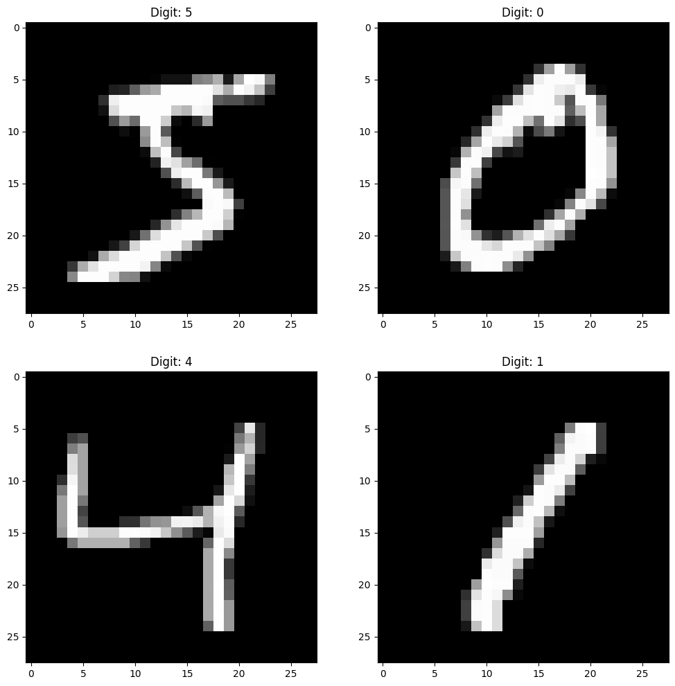
Digital images#
import matplotlib.pyplot as plt
import numpy as np
from sklearn.datasets import fetch_openml
# Fetch MNIST (784 = 28x28 pixels)
mnist = fetch_openml('mnist_784', version=1, as_frame=False)
X, y = mnist.data, mnist.target.astype('int64')
plt.figure(figsize=(12, 12))
plt.subplot(221)
plt.imshow(X[0].reshape(28, 28), cmap='gray')
plt.title(f"Digit: {y[0]}")
plt.subplot(222)
plt.imshow(X[1].reshape(28, 28), cmap='gray')
plt.title(f"Digit: {y[1]}")
plt.subplot(223)
plt.imshow(X[2].reshape(28, 28), cmap='gray')
plt.title(f"Digit: {y[2]}")
plt.subplot(224)
plt.imshow(X[3].reshape(28, 28), cmap='gray')
plt.title(f"Digit: {y[3]}")
# show the plot
plt.show()
Vector-valued functions#
Let \(d,k \in \mathbb{N}\). A vector-valued function of several variables is a function of the form
Thus a vector-valued function \(\pmb{f} = \pmb{x} \mapsto \pmb{f}(\pmb{x})\) has:
Input (domain): vectors \(\pmb{x}\) in \(\mathbb{R}^d\)
Output (codomain): vectors \(\pmb{f}(\pmb{x})\) in \(\mathbb{R}^k\)
Input \(\pmb{x}_0\)#
# Show the third image from the training set
x0 = X[2].reshape(28, 28)
plt.figure(figsize=(7, 7))
plt.imshow(x0, cmap='gray')
plt.axis('off')
plt.show()
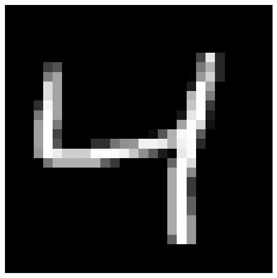
Output \(\pmb{f}(\pmb{x}_0)\)#
Output:
"This is the digit 4"
Ideal output:
This means: "100% sure that this is the digit 4"
More realistic output:
This means: "87% sure that this is the digit 4. Small probability (3%) that it is 1 or 7."
In any case: The output is a vector of probabilities in \(\mathbb{R}^{10}\). Therefore \(\operatorname{co\text{-}dom}(\pmb{f})=\mathbb{R}^{10}\).
What about the input?#
It is actually a matrix of size 28x28:
But it is not immediately a (column) vector!
We can turn it into a vector by stacking the image rows on top of each other. This is called flattening the image in Python.
# Print as a column with 784 numbers
print("\nColumn representation of the image (784 numbers):")
x0.reshape(784,1)
Column representation of the image (784 numbers):
array([[ 0],
[ 0],
[ 0],
[ 0],
[ 0],
[ 0],
[ 0],
[ 0],
[ 0],
[ 0],
[ 0],
[ 0],
[ 0],
[ 0],
[ 0],
[ 0],
[ 0],
[ 0],
[ 0],
[ 0],
[ 0],
[ 0],
[ 0],
[ 0],
[ 0],
[ 0],
[ 0],
[ 0],
[ 0],
[ 0],
[ 0],
[ 0],
[ 0],
[ 0],
[ 0],
[ 0],
[ 0],
[ 0],
[ 0],
[ 0],
[ 0],
[ 0],
[ 0],
[ 0],
[ 0],
[ 0],
[ 0],
[ 0],
[ 0],
[ 0],
[ 0],
[ 0],
[ 0],
[ 0],
[ 0],
[ 0],
[ 0],
[ 0],
[ 0],
[ 0],
[ 0],
[ 0],
[ 0],
[ 0],
[ 0],
[ 0],
[ 0],
[ 0],
[ 0],
[ 0],
[ 0],
[ 0],
[ 0],
[ 0],
[ 0],
[ 0],
[ 0],
[ 0],
[ 0],
[ 0],
[ 0],
[ 0],
[ 0],
[ 0],
[ 0],
[ 0],
[ 0],
[ 0],
[ 0],
[ 0],
[ 0],
[ 0],
[ 0],
[ 0],
[ 0],
[ 0],
[ 0],
[ 0],
[ 0],
[ 0],
[ 0],
[ 0],
[ 0],
[ 0],
[ 0],
[ 0],
[ 0],
[ 0],
[ 0],
[ 0],
[ 0],
[ 0],
[ 0],
[ 0],
[ 0],
[ 0],
[ 0],
[ 0],
[ 0],
[ 0],
[ 0],
[ 0],
[ 0],
[ 0],
[ 0],
[ 0],
[ 0],
[ 0],
[ 0],
[ 0],
[ 0],
[ 0],
[ 0],
[ 0],
[ 0],
[ 0],
[ 0],
[ 0],
[ 0],
[ 0],
[ 0],
[ 0],
[ 0],
[ 0],
[ 0],
[ 0],
[ 0],
[ 0],
[ 0],
[ 0],
[ 0],
[ 0],
[ 0],
[ 0],
[ 0],
[ 0],
[ 0],
[ 0],
[ 0],
[ 0],
[ 67],
[232],
[ 39],
[ 0],
[ 0],
[ 0],
[ 0],
[ 0],
[ 0],
[ 0],
[ 0],
[ 0],
[ 62],
[ 81],
[ 0],
[ 0],
[ 0],
[ 0],
[ 0],
[ 0],
[ 0],
[ 0],
[ 0],
[ 0],
[ 0],
[ 0],
[ 0],
[ 0],
[120],
[180],
[ 39],
[ 0],
[ 0],
[ 0],
[ 0],
[ 0],
[ 0],
[ 0],
[ 0],
[ 0],
[126],
[163],
[ 0],
[ 0],
[ 0],
[ 0],
[ 0],
[ 0],
[ 0],
[ 0],
[ 0],
[ 0],
[ 0],
[ 0],
[ 0],
[ 2],
[153],
[210],
[ 40],
[ 0],
[ 0],
[ 0],
[ 0],
[ 0],
[ 0],
[ 0],
[ 0],
[ 0],
[220],
[163],
[ 0],
[ 0],
[ 0],
[ 0],
[ 0],
[ 0],
[ 0],
[ 0],
[ 0],
[ 0],
[ 0],
[ 0],
[ 0],
[ 27],
[254],
[162],
[ 0],
[ 0],
[ 0],
[ 0],
[ 0],
[ 0],
[ 0],
[ 0],
[ 0],
[ 0],
[222],
[163],
[ 0],
[ 0],
[ 0],
[ 0],
[ 0],
[ 0],
[ 0],
[ 0],
[ 0],
[ 0],
[ 0],
[ 0],
[ 0],
[183],
[254],
[125],
[ 0],
[ 0],
[ 0],
[ 0],
[ 0],
[ 0],
[ 0],
[ 0],
[ 0],
[ 46],
[245],
[163],
[ 0],
[ 0],
[ 0],
[ 0],
[ 0],
[ 0],
[ 0],
[ 0],
[ 0],
[ 0],
[ 0],
[ 0],
[ 0],
[198],
[254],
[ 56],
[ 0],
[ 0],
[ 0],
[ 0],
[ 0],
[ 0],
[ 0],
[ 0],
[ 0],
[120],
[254],
[163],
[ 0],
[ 0],
[ 0],
[ 0],
[ 0],
[ 0],
[ 0],
[ 0],
[ 0],
[ 0],
[ 0],
[ 0],
[ 23],
[231],
[254],
[ 29],
[ 0],
[ 0],
[ 0],
[ 0],
[ 0],
[ 0],
[ 0],
[ 0],
[ 0],
[159],
[254],
[120],
[ 0],
[ 0],
[ 0],
[ 0],
[ 0],
[ 0],
[ 0],
[ 0],
[ 0],
[ 0],
[ 0],
[ 0],
[163],
[254],
[216],
[ 16],
[ 0],
[ 0],
[ 0],
[ 0],
[ 0],
[ 0],
[ 0],
[ 0],
[ 0],
[159],
[254],
[ 67],
[ 0],
[ 0],
[ 0],
[ 0],
[ 0],
[ 0],
[ 0],
[ 0],
[ 0],
[ 14],
[ 86],
[178],
[248],
[254],
[ 91],
[ 0],
[ 0],
[ 0],
[ 0],
[ 0],
[ 0],
[ 0],
[ 0],
[ 0],
[ 0],
[159],
[254],
[ 85],
[ 0],
[ 0],
[ 0],
[ 47],
[ 49],
[116],
[144],
[150],
[241],
[243],
[234],
[179],
[241],
[252],
[ 40],
[ 0],
[ 0],
[ 0],
[ 0],
[ 0],
[ 0],
[ 0],
[ 0],
[ 0],
[ 0],
[150],
[253],
[237],
[207],
[207],
[207],
[253],
[254],
[250],
[240],
[198],
[143],
[ 91],
[ 28],
[ 5],
[233],
[250],
[ 0],
[ 0],
[ 0],
[ 0],
[ 0],
[ 0],
[ 0],
[ 0],
[ 0],
[ 0],
[ 0],
[ 0],
[119],
[177],
[177],
[177],
[177],
[177],
[ 98],
[ 56],
[ 0],
[ 0],
[ 0],
[ 0],
[ 0],
[102],
[254],
[220],
[ 0],
[ 0],
[ 0],
[ 0],
[ 0],
[ 0],
[ 0],
[ 0],
[ 0],
[ 0],
[ 0],
[ 0],
[ 0],
[ 0],
[ 0],
[ 0],
[ 0],
[ 0],
[ 0],
[ 0],
[ 0],
[ 0],
[ 0],
[ 0],
[ 0],
[169],
[254],
[137],
[ 0],
[ 0],
[ 0],
[ 0],
[ 0],
[ 0],
[ 0],
[ 0],
[ 0],
[ 0],
[ 0],
[ 0],
[ 0],
[ 0],
[ 0],
[ 0],
[ 0],
[ 0],
[ 0],
[ 0],
[ 0],
[ 0],
[ 0],
[ 0],
[ 0],
[169],
[254],
[ 57],
[ 0],
[ 0],
[ 0],
[ 0],
[ 0],
[ 0],
[ 0],
[ 0],
[ 0],
[ 0],
[ 0],
[ 0],
[ 0],
[ 0],
[ 0],
[ 0],
[ 0],
[ 0],
[ 0],
[ 0],
[ 0],
[ 0],
[ 0],
[ 0],
[ 0],
[169],
[254],
[ 57],
[ 0],
[ 0],
[ 0],
[ 0],
[ 0],
[ 0],
[ 0],
[ 0],
[ 0],
[ 0],
[ 0],
[ 0],
[ 0],
[ 0],
[ 0],
[ 0],
[ 0],
[ 0],
[ 0],
[ 0],
[ 0],
[ 0],
[ 0],
[ 0],
[ 0],
[169],
[255],
[ 94],
[ 0],
[ 0],
[ 0],
[ 0],
[ 0],
[ 0],
[ 0],
[ 0],
[ 0],
[ 0],
[ 0],
[ 0],
[ 0],
[ 0],
[ 0],
[ 0],
[ 0],
[ 0],
[ 0],
[ 0],
[ 0],
[ 0],
[ 0],
[ 0],
[ 0],
[169],
[254],
[ 96],
[ 0],
[ 0],
[ 0],
[ 0],
[ 0],
[ 0],
[ 0],
[ 0],
[ 0],
[ 0],
[ 0],
[ 0],
[ 0],
[ 0],
[ 0],
[ 0],
[ 0],
[ 0],
[ 0],
[ 0],
[ 0],
[ 0],
[ 0],
[ 0],
[ 0],
[169],
[254],
[153],
[ 0],
[ 0],
[ 0],
[ 0],
[ 0],
[ 0],
[ 0],
[ 0],
[ 0],
[ 0],
[ 0],
[ 0],
[ 0],
[ 0],
[ 0],
[ 0],
[ 0],
[ 0],
[ 0],
[ 0],
[ 0],
[ 0],
[ 0],
[ 0],
[ 0],
[169],
[255],
[153],
[ 0],
[ 0],
[ 0],
[ 0],
[ 0],
[ 0],
[ 0],
[ 0],
[ 0],
[ 0],
[ 0],
[ 0],
[ 0],
[ 0],
[ 0],
[ 0],
[ 0],
[ 0],
[ 0],
[ 0],
[ 0],
[ 0],
[ 0],
[ 0],
[ 0],
[ 96],
[254],
[153],
[ 0],
[ 0],
[ 0],
[ 0],
[ 0],
[ 0],
[ 0],
[ 0],
[ 0],
[ 0],
[ 0],
[ 0],
[ 0],
[ 0],
[ 0],
[ 0],
[ 0],
[ 0],
[ 0],
[ 0],
[ 0],
[ 0],
[ 0],
[ 0],
[ 0],
[ 0],
[ 0],
[ 0],
[ 0],
[ 0],
[ 0],
[ 0],
[ 0],
[ 0],
[ 0],
[ 0],
[ 0],
[ 0],
[ 0],
[ 0],
[ 0],
[ 0],
[ 0],
[ 0],
[ 0],
[ 0],
[ 0],
[ 0],
[ 0],
[ 0],
[ 0],
[ 0],
[ 0],
[ 0],
[ 0],
[ 0],
[ 0],
[ 0],
[ 0],
[ 0],
[ 0],
[ 0],
[ 0],
[ 0],
[ 0],
[ 0],
[ 0],
[ 0],
[ 0],
[ 0],
[ 0],
[ 0],
[ 0],
[ 0],
[ 0],
[ 0],
[ 0],
[ 0],
[ 0],
[ 0],
[ 0],
[ 0],
[ 0],
[ 0],
[ 0],
[ 0],
[ 0],
[ 0],
[ 0],
[ 0],
[ 0],
[ 0]])
So we can think of the input as vectors in \(\mathbb{R}^{784}\)! That is,
An AI function#
The AI is a vector-valued function with \(d=784\), \(k=10\).
In machine learning, the function is called a model, and the specific AI function typically depends on thousands or millions of parameters (called weights). For each set of parameters/weights we get a new AI function. Such functions (also deep neural networks) are not particularly complicated, but often long to write explicitly. They are built from
Composition of simple vector-valued functions \(\pmb{g} \circ \pmb{h}\)
The simple functions are usually only: 1. Affine vector-valued functions \(\pmb{x} \mapsto A \pmb{x} + \pmb{b}\) (the elements of the matrix \(A\) and the vector \(\pmb{b}\) are the parameters/weights) 2. A non-linear activation function, e.g. ReLU.
The number of compositions \(\pmb{g}_1 \circ \pmb{g}_2 \circ \pmb{g}_3 \circ \cdots \circ \pmb{g}_N\) describes the network’s depth.
Neural networks#
What do these “AI functions” look like?
General notation for a feedforward ReLU network#
A feedforward network computes the output by sequentially passing the input through a series of layers. For each layer \(\ell\), we first compute a pre-activation (also called logits), \(z^{(\ell)}\), followed by an activation (or hidden state), \(h^{(\ell)}\).
where
\(h^{(0)}\) is the input vector \(x\).
\(W_\ell \in \mathbb{R}^{n_\ell \times n_{\ell-1}}\) is the weight matrix for layer \(\ell\).
\(b_\ell \in \mathbb{R}^{n_\ell}\) is the bias vector.
\(\sigma:\mathbb{R}\to\mathbb{R}\) is a non-linear activation function (applied coordinate-wise), typically ReLU:
\(n_0=d\) is the input dimension, \(n_L=k\) the output dimension.
We say briefly that the network is of the form \(n_0 \to n_1 \to \cdots \to n_L\).
The network’s overall function \(\Phi: \mathbb{R}^d \to \mathbb{R}^k\) gives the final output:
since the last layer here is linear (without ReLU activation).

General formula for a ReLU network with \(L=3\)#
We consider a function
defined as a fully connected network with two hidden layers:
where \(n_0 = d\), \(n_3 = k\), and
\(W_1 \in \mathbb{R}^{n_1\times n_0},\ b_1\in\mathbb{R}^{n_1}\)
\(W_2 \in \mathbb{R}^{n_2\times n_1},\ b_2\in\mathbb{R}^{n_2}\)
\(W_3 \in \mathbb{R}^{n_3\times n_2},\ b_3\in\mathbb{R}^{n_3}\)
The overall functional expression becomes:
Example: For a concrete network with two input variables and one output of the form \(2 \to n_1 \to n_2 \to 1\):
where the dimensions are
Networks and training directly in SKLearn#
We want to find an “AI function”
that can classify an image of a handwritten digit as well as possible.
In the code below, this is built as a ReLU network with two hidden layers, giving a total depth of \(L=3\). The shape of the network is \(784 \to 256 \to 128 \to 10\). Thus the weight matrices have sizes
from sklearn.model_selection import train_test_split
from sklearn.neural_network import MLPClassifier

# Normalize to [0,1]
X = X / 255.0

X_train, X_test, y_train, y_test = train_test_split(
    X, y, test_size=1/7, random_state=42
)

# DNN with the same “size” as the PyTorch example
clf = MLPClassifier(
    hidden_layer_sizes=(256, 128),  # two hidden layers
    activation='relu',
    solver='adam',
    batch_size=64,
    learning_rate_init=1e-3,
    max_iter=6,
    verbose=True
)
Network size#
How many parameters are there?
Answer#
The total number of parameters for the network is:
Layer 1: (784 inputs × 256 neurons) + 256 biases = 200.704 + 256 = 200.960
Layer 2: (256 inputs × 128 neurons) + 128 biases = 32.768 + 128 = 32.896
Layer 3: (128 inputs × 10 neurons) + 10 biases = 1.280 + 10 = 1.290
Total: 200.960 + 32.896 + 1.290 = 235.146
Training via SKLearn#
We find the optimal values of all parameters in the \(\Phi\) function by training the model with the fit method:
# Train
clf.fit(X_train, y_train)
Iteration 1, loss = 0.23305379
Iteration 2, loss = 0.08945422
Iteration 3, loss = 0.05943136
Iteration 4, loss = 0.04277573
/builds/ctm/ctmweb/venv/lib/python3.11/site-packages/sklearn/neural_network/_multilayer_perceptron.py:792: UserWarning: Training interrupted by user.
  warnings.warn("Training interrupted by user.")
MLPClassifier(batch_size=64, hidden_layer_sizes=(256, 128), max_iter=6,
              verbose=True)
In a Jupyter environment, please rerun this cell to show the HTML representation or trust the notebook. On GitHub, the HTML representation is unable to render, please try loading this page with nbviewer.org.
Parameters
Prediction on a single image#
We can now use this function on a single input image to get a prediction. Let’s take a single image from our test set and see what the model predicts.
image_index = 2 # Choose an image (input)
input_image = X_test[image_index:image_index+1] # Format (1, 784)
true_label = y_test[image_index]

probability_vector = clf.predict_proba(input_image) # Get the probability vector
predicted_label = clf.predict(input_image) # Make prediction

print(input_image)
print(true_label)
print(probability_vector)
print(predicted_label)
Overall prediction#
The overall percentage of images in the test set that the model classified correctly can be found by:
# Overall evaluation
print("Test accuracy:", clf.score(X_test, y_test))
Visualization of predictions#
To get a better sense of how the model behaves, we can visualize its predictions on individual images from the test set. The function below plots the image, the true label, the predicted label, and a bar chart of the predicted probabilities for each class. This is useful for seeing when the model is confident and when it is uncertain.
def show_images_with_mlp_probabilities(clf, X_test, y_test, X_test_orig,
                                       num_images=5, only_incorrect=False,
                                       image_shape=(8,8)):
    # Predict full test set
    pred_labels = clf.predict(X_test)
    probas = clf.predict_proba(X_test)

    # Select indices
    all_indices = np.arange(len(X_test))
    if only_incorrect:
        indices = all_indices[pred_labels != y_test][:num_images]
    else:
        indices = all_indices[:num_images]

    plt.figure(figsize=(12, 6))

    for i, idx in enumerate(indices):
        # --- Image plot ---
        plt.subplot(2, num_images, i + 1)
        img = X_test_orig[idx].reshape(image_shape)
        plt.imshow(img, cmap='gray')
        plt.title(f"Idx {idx}\nTrue {y_test[idx]}\nPred {pred_labels[idx]}")
        plt.axis('off')

        # --- Probability distribution ---
        plt.subplot(2, num_images, num_images + i + 1)

        p = probas[idx]

        classes = np.arange(len(p))
        colors = [
            "red" if c == y_test[idx] else
            ("green" if c == pred_labels[idx] else "blue")
            for c in classes
        ]

        plt.bar(classes, p, color=colors)
        plt.xticks(classes)
        plt.ylim(0, 1)
        plt.xlabel("Class")
        plt.ylabel("Probability")

    plt.tight_layout()
    plt.show()

show_images_with_mlp_probabilities(
    clf,
    X_test,
    y_test,
    X_test_orig=X_test,
    only_incorrect=False,
    num_images=5,
    image_shape=(28,28)
)
show_images_with_mlp_probabilities(
    clf,
    X_test,
    y_test,
    X_test_orig=X_test,
    only_incorrect=True,
    num_images=5,
    image_shape=(28,28)
)