import matplotlib
if not hasattr(matplotlib.RcParams, "_get"):
    matplotlib.RcParams._get = dict.get

Neural Networks and Digital Images

0: Setup

import numpy as np
np.random.seed(0)
from mpl_toolkits.mplot3d import Axes3D

import matplotlib
if not hasattr(matplotlib.RcParams, "_get"):
    matplotlib.RcParams._get = dict.get
import matplotlib.pyplot as plt

from sklearn.model_selection import train_test_split
from skimage import data, img_as_float, restoration, color, util
from sklearn.datasets import load_digits
from sklearn.preprocessing import OneHotEncoder
from scipy import fftpack, ndimage, linalg
from sympy import symbols
from sympy.plotting import plot3d

plt.rcParams["figure.figsize"] = (6,4)
np.set_printoptions(precision=4, suppress=True)

1: Digital image as a matrix

We import an image:

img = img_as_float(data.camera())
plt.imshow(img, cmap="gray", vmin=0, vmax=1); plt.axis("off"); plt.title("Grayscale image")

Text(0.5, 1.0, 'Grayscale image')

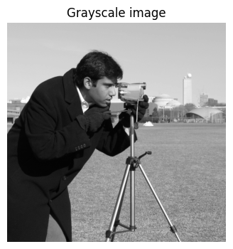
How do you view this image as a matrix in Python? What is the size of the matrix, which values are included in the matrix, and what do the values in the matrix represent?

# Convert to numpy array and inspect size
# Add CODE HERE

Answer

The values in the matrix are decimal numbers normalized to the interval [0, 1], where each value represents the grayscale intensity of the corresponding pixel (0 = black, 1 = white). The matrix dimensions correspond to the image’s height and width (512×512).

You can copy-paste this code into a Python window:

# Convert to numpy array and inspect size

arr = np.array(img)
print("shape:", arr.shape, "dtype:", arr.dtype)

Zoom in on the \(8 \times 8\) pixels in the top-left corner and print the pixel values as an \(8 \times 8\) matrix. What do you notice about the 64 grayscale values?

print("Top-left 8×8 block:")
# ADD CODE HERE

Top-left 8×8 block:

Answer

It is observed that the 64 grayscale values in the top-left corner are almost constant, indicating a homogeneous region without many details (e.g., a “uniform” surface). This is also seen in the zoomed image, where neighboring pixels vary only slightly, indicating low local contrast in that region. In general, for most natural high-resolution images, there is a high degree of spatial correlation: the value of a pixel is often very close to the value of its neighboring pixels. This redundancy (excess information) is a fundamental property exploited in image compression formats such as JPEG. Instead of storing the exact value for each pixel, it is more efficient to store a base value and the small differences to neighboring pixels.

print("Top-left 8×8 block:")
print(arr[:8, :8])

plt.imshow(arr[:8, :8], cmap="gray", vmin=0, vmax=1); plt.axis("off"); plt.title("Zoomed image")

Now zoom in on the \(8 \times 8\) pixels in the bottom-right corner and show your zoom as a (pixelated) image

# ADD CODE HERE

Answer

print("Bottom-right 8×8 block:")
print(arr[-8:, -8:])

plt.imshow(arr[-8:, -8:], cmap="gray", vmin=0, vmax=1); plt.axis("off"); plt.title("Zoomed image")

2: Digital image as a vector

We will work with automatic recognition of handwritten digits from sklearn.datasets.load_digits:

digits_object = load_digits() 
X = digits_object.data  # fetch data
y = digits_object.target # fetch labels
X = X / 16.0  # normalize to [0, 1]

# Show some examples
fig, axes = plt.subplots(2, 5, figsize=(8, 3))
for ax, img, label in zip(axes.ravel(), X, y):
    ax.imshow(img.reshape(8, 8), cmap="gray", vmin=0, vmax=1)
    ax.set_title(f"Label: {label}")
    ax.axis("off")

plt.show()

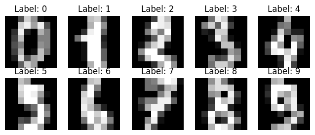
Can you see which handwritten digits are shown? Check with the correct labels.

Today, we would like to build a neural network \(\Phi : \mathbb{R}^n \to \mathbb{R}^k\) that can recognize these handwritten digits. This “AI function” thus takes a vector in \(\mathbb{R}^n\) as input and outputs a vector in \(\mathbb{R}^k\).

Our input is initially an \(8 \times 8\) matrix:

example_img = X[0].reshape(8, 8)  # image as 8x8 matrix
print(example_img)

[[0.     0.     0.3125 0.8125 0.5625 0.0625 0.     0.    ]
 [0.     0.     0.8125 0.9375 0.625  0.9375 0.3125 0.    ]
 [0.     0.1875 0.9375 0.125  0.     0.6875 0.5    0.    ]
 [0.     0.25   0.75   0.     0.     0.5    0.5    0.    ]
 [0.     0.3125 0.5    0.     0.     0.5625 0.5    0.    ]
 [0.     0.25   0.6875 0.     0.0625 0.75   0.4375 0.    ]
 [0.     0.125  0.875  0.3125 0.625  0.75   0.     0.    ]
 [0.     0.     0.375  0.8125 0.625  0.     0.     0.    ]]

How can we convert it into a vector?

# ADD CODE HERE

Answer

# flatten matrix into vector
example_img = X[0].reshape(8, 8)  # first image as 8x8 matrix
example_vec = example_img.flatten()  # flatten to vector of length 64

print("Matrix shape:", example_img.shape)
print("Vector shape:", example_vec.shape)
example_img, example_vec

The input to our AI function \(\Phi\) is handwritten digits (represented as a vector in \(\mathbb{R}^n\)). We want the output of \(\Phi\) to be a probability vector of length 10, with the probability that the handwritten digit is respectively 0, 1, 2, …, 9.

Note

A probability vector is a vector of numbers belonging to [0,1], whose elements sum to 1 (i.e., a discrete probability distribution over the classes).

What are \(n\) and \(k\) in our example? What is the ideal output of the function \(\Phi\) if the input is a handwritten 8?

Answer

n = 64 (8×8 pixels flattened) k = 10 (the classes 0–9)

Ideal output for a handwritten 8: a “one-hot” probability vector of length 10 with 1 at index 8, e.g. [0,0,0,0,0,0,0,0,1,0] (remember we use 0-based indexing — thus the 1 is placed at index 8 (the ninth component)

The (so far unknown) AI function \(\Phi\) is built as a neural network. The next exercises introduce the building blocks of such functions.

3: The ReLU function

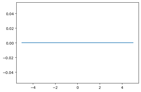
Define the ReLU function \(\mathrm{ReLU}: \mathbb{R} \to \mathbb{R}\) in Python. Plot the graph of the function.

def relu(z):
    return 0 * z # FIX CODE HERE

x = np.linspace(-5, 5, 200)
plt.plot(x, relu(x), label="ReLU")

[<matplotlib.lines.Line2D at 0x7f60a27a22d0>]

Answer

def relu(z):
    return np.maximum(0.0, z)

Explain what happens in the following code.

vec = np.array([-3, -1, 0, 1, 3])
print("ReLU on vector:", relu(vec)) 

ReLU on vector: [0 0 0 0 0]

Answer

ReLU is defined as a scalar function of one variable, but we can easily extend it to a vector function by letting it act on a vector coordinate-wise, which Python does completely automatically.

Is the ReLU function linear? Is it continuous? Compute its derivative. Is it differentiable?

Hint

A linear function satisfies \(f(x+y)=f(x)+f(y)\) and \(f(a x)=a f(x)\) for all \(x,y\) and all scalars \(a\).

Answer

ReLU is not linear: for example it does not satisfy \(f(-1)=-f(1)\).

ReLU is continuous (no jumps), but only piecewise linear. The derivative is

• \(f'(x)=0\) for \(x<0\)

• \(f'(x)=1\) for \(x>0\) and it is not differentiable at \(x=0\) (the function’s only non-differentiable point). (It is possible to talk about a subgradient at \(x=0\), which can be any number in [0,1].)

4: The Gradient

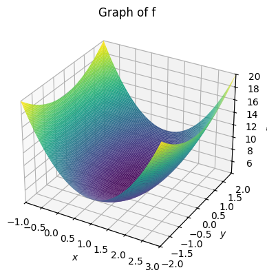
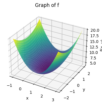
We want to find the minimum of a function

\[\begin{equation*} f:\mathbb{R}^2 \to \mathbb{R}, \qquad f(x,y) = 3(x-1)^2 + y^2 + 4. \end{equation*}\]

We first plot the graph of the function. In SymPy this is done by:

# Define the symbols x and y
x, y = symbols('x, y')

# Define the function f(x,y)
f = 3*(x-1)**2 + y**2 + 4

# Plot the function as a 3D surface
plot3d(f, (x, -1, 3), (y, -2, 2), title="Graph of f")

<sympy.plotting.backends.matplotlibbackend.matplotlib.MatplotlibBackend at 0x7f60a2644490>

while in NumPy it requires a bit more work:

# Define the function f(x,y)
def f(x, y):
    return 3*(x-1)**2 + y**2 + 4

# Create a grid of (x, y) values
x_vals = np.linspace(-1, 3, 100)
y_vals = np.linspace(-2, 2, 100)
X, Y = np.meshgrid(x_vals, y_vals)

# Calculate the Z values for each point in the grid
Z = f(X, Y)

# Create the 3D plot
fig = plt.figure()
ax = fig.add_subplot(111, projection='3d')

# Plot the surface
ax.plot_surface(X, Y, Z, cmap='viridis', edgecolor='none')

# Add titles and labels
ax.set_title("Graph of f")
ax.set_xlabel('x')
ax.set_ylabel('y')
ax.set_zlabel('f(x, y)')

plt.show()

a: The gradient vector

We consider the function \(f : \mathbb{R}^2 \to \mathbb{R}\) given by:

\[\begin{equation*} f(x,y)=3(x-1)^2 + y^2 + 4 \end{equation*}\]

The gradient vector consists of the partial derivatives:

\[\begin{equation*} \nabla f(x,y) = \begin{bmatrix} \frac{\partial f}{\partial x} \\ \frac{\partial f}{\partial y} \end{bmatrix}. \end{equation*}\]

which can also be written as \(\nabla f(x,y) = [\frac{\partial f}{\partial x}, \frac{\partial f}{\partial y}]^T\) — here, the T simply means we take the transpose of the row vector, which turns it into a column vector.

Find the gradient vector for \(f\).

Answer

Compute:

\[\begin{equation*} \frac{\partial f}{\partial x} = 6(x-1),\qquad \frac{\partial f}{\partial y} = 2y. \end{equation*}\]

Thus:

\[\begin{equation*} \nabla f(x,y) = \begin{bmatrix} 6(x-1)\\[4pt] 2y \end{bmatrix}. \end{equation*}\]

b: The gradient vector and level curves

Plot the gradient vector at an arbitrary point \((x_0,y_0)\). Plot the level curve through the same point.

# ADD CODE HERE

Note

Level curves for a function \(f\) are the set of points \((x,y)\) where \(f(x,y)=c\) for a given real number \(c\), and in Python you can create a grid over the (x,y)-plane with:

x = np.linspace( -1.0, 4.0, 200)
y = np.linspace( -2.0, 2.5, 200)
Xg, Yg = np.meshgrid(x, y)
Z = f(Xg, Yg)

and use matplotlib.pyplot.contour or contourf to draw level curves: plt.contour(Xg, Yg, Z, levels=15, cmap="gray") One typically plots several level curves in the same plot.

It can take time to write the code to plot these things from scratch. Once you have made an attempt, or if you get stuck, you are welcome to use the code in the answer as inspiration or to move forward.

Answer

def f(x, y):
    return 3*(x-1)**2 + y**2 + 4

def grad(x, y):
    return np.array([6*(x-1), 2*y])

# Choose a point (x0,y0)
x0, y0 = 2.0, 1.0
g = grad(x0, y0)

# Grid for contour plot
x = np.linspace( -1.0, 4.0, 200)
y = np.linspace( -2.0, 2.5, 200)
Xg, Yg = np.meshgrid(x, y)
Z = f(Xg, Yg)

# Contour level through the chosen point
c_level = f(x0, y0)

plt.figure(figsize=(6,6))
# Plot several level curves
cs = plt.contour(Xg, Yg, Z, levels=15, cmap="gray")
plt.clabel(cs, inline=True, fontsize=8)

# Highlight the specific level curve through (x0,y0)
plt.contour(Xg, Yg, Z, levels=[c_level], colors="red", linewidths=2, linestyles="--")

# Plot the point and gradient vectors (gradient and negative gradient)
plt.plot(x0, y0, "ko", label=f"point ({x0},{y0})")
# scale arrows for visibility
scale = 0.25
plt.arrow(x0, y0,  scale*g[0],  scale*g[1], color="blue",
          head_width=0.08, head_length=0.1, length_includes_head=True, label="grad f")
plt.arrow(x0, y0, -scale*g[0], -scale*g[1], color="green",
          head_width=0.08, head_length=0.1, length_includes_head=True, label="-grad f")

plt.text(x0 + 0.05, y0 + 0.05, f"∇f={g}", fontsize=9)
plt.axis("equal")
plt.xlabel("x"); plt.ylabel("y")
plt.title("Gradient at point and level curve through the point")
plt.legend(["point", "gradient (blue)", "negative gradient (green)"], loc="upper left")
plt.show()

c: Minimum

At which point \((x,y)\) does the function attain its minimum value?

Answer

From the graph of the function we can see that the function has a minimum, and from the plot of the level curves one can read off where the function attains its minimum value. One can also “compute” it: At such a minimum point there is no direction in which the function increases, and therefore the gradient vector must be the zero vector. We can thus find the minimum by solving the equation \(\nabla f(x,y) = \mathbf{0}\).

This gives us the two equations:

\[\begin{equation*} 6(x-1)=0 \quad \text{and} \quad 2y=0 \end{equation*}\]

The only solution to these equations is the point \((x,y)=(1,0)\). This is therefore the function’s minimum point.

Points where the gradient vector is the zero vector are called stationary points, and such points can be (local) minima, maxima, or so-called saddle points.

d: Interpretation

How should one understand (the correct) statement: “The gradient \(\nabla f(x,y)\) points in the direction (from the point \((x,y)\)) where the function increases fastest”? Is it correct that \(-\nabla f(x,y)\) points in the direction where the function decreases fastest?

Answer

Yes, both statements are correct. The gradient \(\nabla f(x,y)\) is a vector in the \((x,y)\)-plane that points in the direction one should move to achieve the fastest increase in the function value. Conversely, the negative gradient, \(-\nabla f(x,y)\), points in the direction of the fastest decrease.

It is important to remember that the gradient only provides local information. It tells us about the steepest direction exactly at the point we are at (based on the tangent plane at the point).

Example: For the function \(f(x,y) = 3(x-1)^2 + y^2 + 4\) at the point \((x,y)=(2,1)\) the gradient is \(\nabla f(2,1) = [6, 2]^T\). The negative gradient is therefore \(-\nabla f(2,1) = [-6, -2]^T\). If we are at the point \((2,1)\) and want to find the function’s minimum, the locally best direction to move is in the direction \([-6, -2]^T\) (or any positive scaling of it, e.g. \([-3, -1]^T\)). We do not, however, know how far we should move in this direction.

Does the negative gradient always point exactly toward the function’s minimum?

Answer

No. The negative gradient only points in the local direction of steepest descent and provides no global information.

5: The Gradient Method

The concept of “Training an AI”, as often mentioned e.g. in the media, covers a fundamental optimization process. The core of this process is the gradient method. In English it is often referred to as “gradient descent”; in practice one typically uses a stochastic variant called stochastic gradient descent (SGD).

a: Mountain climbing with the gradient vector

We imagine that the graph of the function

\[\begin{equation*} B(x,y)=4000-3(x-10)^2 - (y-3)^2 \end{equation*}\]

forms a mountain we want to climb (so we want to find the maximum of the function). We are located at the point \((x_0,y_0)=(0,0)\) — or to be more precise, at the point \((x_0,y_0, B(x_0,y_0))=(0,0, 3691)\). It is very foggy, so we can only see one meter around our feet, and thus we cannot see where the summit is. We can compute the gradient vector at the point we are at.

Devise a method to iteratively approach the summit.

Answer

An iterative method, often called “hill climbing” or gradient ascent, can be used:

1. Starting position: We start at the point \((x_0, y_0) = (0,0)\).

2. Find the direction: At our current position, we compute the gradient vector \(\nabla B(x,y)\). This vector points in the direction where the mountain increases most steeply.

3. Take a step: We take a small step in the direction the gradient points. The step size should be small enough that we do not risk going too far (e.g., “overshooting” the summit).

4. Repeat: We repeat the process from our new position: compute the gradient, take another small step uphill, and continue.

For each step, we will move higher up the mountain. We can stop when the steps we take become very small, which indicates that we are close to the summit, where the terrain flattens out (and the gradient approaches zero).

Bonus question (which is not important for the exercise): From the function expression, can you see how tall the mountain is?

b: Min or max? Plus or minus the gradient?

The gradient method is an iterative algorithm that moves in:

1. the minus gradient direction

2. the (plus) gradient direction

to find

1. a (local) maximum

2. a (local) minimum

Pair the lists above to form (two) correct statements.

Answer

If the goal is to find:	Then move in:
(local) minimum	minus gradient direction
(local) maximum	plus gradient direction

c: The Gradient Method

One step in the method is given by

\[\begin{equation*} \begin{bmatrix} x_{k+1}\\[4pt] y_{k+1} \end{bmatrix} = \begin{bmatrix} x_k\\[4pt] y_k \end{bmatrix} - \eta\,\nabla B(x_k,y_k), \end{equation*}\]

where \(\eta>0\) is called the learning rate (or step size).

When one repeats this step with a suitable \(\eta\), \((x_k,y_k)\) will converge toward \((10,3)\).

Discuss what the size of \(\eta\) does. What does \(\eta=1\) correspond to? Is it an appropriate size?

Answer

\(\eta=1\) corresponds to taking a full “gradient step” (moving by the entire gradient vector without scaling). This gives a very large step and can easily lead to an unstable algorithm. The size of \(\eta\) determines speed vs. stability: for small \(\eta\) you converge slowly but stably, for too large \(\eta\) you get oscillations (e.g., if you take an overly long step to the other side of the mountain). In machine learning one typically chooses \(\eta \approx 0.001\) or even smaller, especially if the network landscape is very complicated. One cannot make a general rule for choosing \(\eta\), and it is often chosen based on experience or observations.

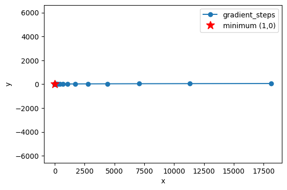
d: Python example

Below, the gradient method is shown for the function in Exercise 4: The Gradient.

def f(x, y):
    return 3*(x-1)**2 + y**2 + 4

def grad(x, y):
    return np.array([6*(x-1), 2*y])

# initial point and learning rate
x = np.array([2.5, 1.5], dtype=float)
eta = 0.1

path = [x.copy()]

# 20 iterations/steps
for _ in range(20):  
    x = x + eta * grad(*x)
    path.append(x.copy())

path = np.array(path)
plt.plot(path[:,0], path[:,1], 'o-', label='gradient_steps')
plt.plot(1,0,'r*',markersize=12,label='minimum (1,0)')
plt.xlabel('x'); plt.ylabel('y'); plt.axis('equal'); plt.legend(); plt.show()

Make a similar plot for the function (the mountain \(B\)) in this exercise. Try different values of \(\eta\), initial guesses, and number of iterations. (Remember that now we are not looking for a minimum, but a maximum. Be careful not to go “the wrong way”.)

e: A remark on training

Let us return to the exercise introduction: “The concept of “Training AI”, as often mentioned in the media, covers a fundamental optimization process. The core of this process is the gradient method”

Imagine a loss function that measures how “wrong” an AI model’s predictions are compared to the correct data. The goal of training is to find the values for the model’s parameters (i.e., weights and biases, \(W\) and \(b\), introduced in the next exercise) that make this loss function as small as possible.

The gradient method is the algorithm that systematically adjusts these thousands or millions of parameters. At each step, it computes the gradient of the loss function with respect to the model’s parameters and moves the parameters in the negative gradient direction — exactly as we moved in the simple 2D example. In this way, the model “learns” to become more accurate.

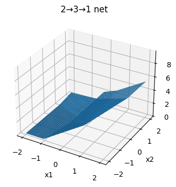
6: The Network Landscape: The Graph of a Neural Network

In this exercise we will visualize and interpret piecewise linear functions created by ReLU networks, where the input dimension is \(2\) and the output dimension is \(1\). These are functions of the form \(\Phi: \mathbb{R}^2 \to \mathbb{R}\). The graph of a neural network (the network function \(\Phi\)) is called the network landscape.

Here we only consider shallow networks, where there is only one hidden layer. The architecture of our network can be described with the notation \(2 \to n \to 1\) (or as \(\mathbb{R}^2 \to \mathbb{R}^n \to \mathbb{R}^1\)). This notation indicates the number of neurons in each layer:

• 2 neurons in the input layer, corresponding to the two input variables \((x_1, x_2)\) which form a (column) vector in \(\mathbb{R}^2\).

• \(n\) neurons in the hidden layer, whose output can be thought of as a column vector in \(\mathbb{R}^n\). This number, \(n\), can be varied to see how it affects the network’s complexity.

• 1 neuron in the output layer, which produces the final output value \(z=\Phi(x_1, x_2)\), which here is just a number in \(\mathbb{R}^1\). In the output layer one typically uses no activation function such as ReLU, since ReLU would make negative output values impossible.

We need to understand the relationship between the number of neurons in the hidden layer, \(n\), and the “complexity” of the network landscape.

The neural network is built from the following functions:

def relu(z):
    return np.maximum(0.0, z)

def sample_weights(n):
    W1 = np.random.randn(n, 2)
    b1 = 0.2 * np.random.randn(n, 1)
    W2 = np.random.randn(1, n)
    b2 = 0.2 * np.random.randn(1, 1)
    return W1, b1, W2, b2

def neural_network(W1, b1, W2, b2, X):  
    Z1 = W1 @ X + b1  # Pre-activation (logits) for hidden layer
    H = relu(Z1)      # Post-activation for hidden layer
    Z2 = W2 @ H + b2  # Final output (logits)
    return Z2

Finally, we introduce some helper functions to plot the graph:

# 2D grid evaluation 
def eval_on_grid(W1, b1, W2, b2, xlim=(-2,2), ylim=(-2,2), res=120):
    x1_vals = np.linspace(xlim[0], xlim[1], res)
    x2_vals = np.linspace(ylim[0], ylim[1], res)
    X1g, X2g = np.meshgrid(x1_vals, x2_vals, indexing='xy')
    XY_grid = np.stack([X1g.ravel(), X2g.ravel()], axis=0)      # (2, res*res)
    Z_out = neural_network(W1, b1, W2, b2, XY_grid).reshape(X1g.shape) # (res, res)
    return X1g, X2g, Z_out

# Plots 
def plot_surface(W1, b1, W2, b2, title="", xlim=(-2,2), ylim=(-2,2), res=120):
    X1g, X2g, Z_out = eval_on_grid(W1, b1, W2, b2, xlim, ylim, res)
    fig = plt.figure()
    ax = fig.add_subplot(111, projection='3d')
    ax.plot_surface(X1g, X2g, Z_out, linewidth=0, antialiased=True)
    ax.set_title(title)
    ax.set_xlabel("x1")
    ax.set_ylabel("x2")
    ax.set_zlabel("Φ(x1,x2)")
    plt.show()

def plot_contours(W1, b1, W2, b2, levels=10, title="", xlim=(-2,2), ylim=(-2,2), res=200):
    X1g, X2g, Z_out = eval_on_grid(W1, b1, W2, b2, xlim, ylim, res)
    plt.figure()
    cs = plt.contour(X1g, X2g, Z_out, levels=levels)
    plt.clabel(cs, inline=True, fontsize=8)
    plt.title(title if title else "Contour of Φ")
    plt.xlabel("x1"); plt.ylabel("x2")
    plt.axis("equal")
    plt.show()

a: The network when n=3

Build a network of the form (\(2\to 3\to 1\)) in Python, where you choose the following weights:

\[\begin{equation*} W_1 = \begin{bmatrix} 1 & -1\\[4pt] 2 & 0\\[4pt] -1 & 2 \end{bmatrix},\qquad b_1 = \begin{bmatrix} 0\\[4pt] 1\\[4pt] -1 \end{bmatrix},\qquad W_2 = \begin{bmatrix} 1 & -2 & 1 \end{bmatrix},\qquad b_2 = \begin{bmatrix} 0 \end{bmatrix}. \end{equation*}\]

Note

The word “weights” is used here simply to refer to the parameters (the numbers) in the matrices \(W_\ell\) and the vectors \(b_\ell\). Normally, \(W_\ell\) is called “the weight matrix” while \(b_\ell\) is called “the bias”. These are the parameters one changes when training a network using the gradient method.

Check that your network returns the value \(-4\) when you call neural_network(W1, b1, W2, b2, np.array([[1.],[-1.]])). Then plot the graph as a 3D surface \(z=\Phi(x_1,x_2)\) for the network with exactly these \(W_\ell\) matrices and \(b_\ell\) vectors. Below, the graph for a “random” network is plotted:

# Sample random weights for a 2 -> 3 -> 1 network
W1, b1, W2, b2 = sample_weights(3)

# Single test input (column vector)
x_test = np.array([[1.],[-1.]])   # shape (2,1)
z2_test = neural_network(W1, b1, W2, b2, x_test)
print("neural_network output for x = [[1.],[-1.]] ->", z2_test.ravel())

# A few more test points (shape (2, N))
X_check = np.array([[0., 1., 0., 1.],
                    [0., 0., 1., 1.]])
z2_check = neural_network(W1, b1, W2, b2, X_check)
print("inputs:", X_check.T)
print("outputs:", z2_check.ravel())

# Visualize using the helper functions already defined above
plot_surface(W1, b1, W2, b2, title="2→3→1 net")
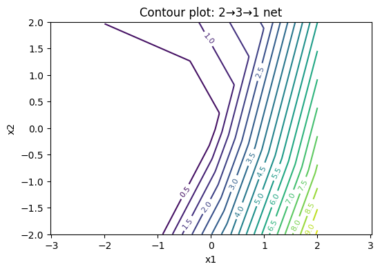
plot_contours(W1, b1, W2, b2, levels=20, title="Contour plot: 2→3→1 net")

neural_network output for x = [[1.],[-1.]] -> [4.8974]
inputs: [[0. 0.]
 [1. 0.]
 [0. 1.]
 [1. 1.]]
outputs: [0.2302 3.7771 0.713  2.8429]

Answer

# Deterministic integer weights for a 2 -> 3 -> 1 network
W1 = np.array([[ 1., -1.],
               [ 2.,  0.],
               [-1.,  2.]])
b1 = np.array([[0.],[1.],[-1.]])
W2 = np.array([[1., -2., 1.]])
b2 = np.array([[0.]])

How many “kinks” can you see in the level curves? Why is the surface piecewise planar? How many linear pieces is the surface composed of?

Answer

You should be able to see (up to) three “kinks” in each level curve. Each kink comes from exactly one neuron in the hidden layer.

1. Why does a “kink” occur?

2. Why is the surface piecewise planar?

3. What is the number of regions?

Answer to 1. Each neuron, \(k\), in the hidden layer first computes a linear function of the input: \(\mathbf{w_k} \cdot \mathbf{x} + b_k\). The result of this computation is sent into the ReLU function. Since \(\text{ReLU}\) is only active for positive values, the neuron “turns on” or “turns off” at the boundary where its input is zero. This boundary is a line in the input plane, defined by the equation:

\[ \mathbf{w}_k \cdot \mathbf{x} + b_k = 0 \]

When the input point \(\mathbf{x}\) crosses this line, the output from that neuron changes abruptly from \(0\) to a linear function (or vice versa). This creates a “kink” in the overall function. With \(n=3\) neurons, there are thus three such lines that create kinks in the surface.

Answer to 2. The \(n\) lines divide the input plane into different regions. Within any of these regions, the activation pattern for all neurons is fixed (each neuron is either constantly “on” or constantly “off”). When the activation pattern is fixed, the entire network behaves as a simple affine function (a linear transformation plus a constant). The graph of an affine function is a plane. Therefore, the network’s overall graph consists of different planar “pieces” that are joined at the kink lines.

Answer to 3. Number of regions: With \(n=3\) lines, the plane can be divided into at most 7 different linear regions. This is a classic result from combinatorial geometry. Try drawing 3 random lines on a piece of paper and count the number of regions between the lines.

b: The network when n is lower and higher

Run the same visualization for \(n=1\) and \(n=8\) and compare the visual complexity of the graph for the network \(\Phi(x_1,x_2)\). The restriction of the function \(\Phi(x_1,x_2)\) along a line in the plane \(x_2 = a x_1 + b\) will be a piecewise linear function of one variable, namely \(x_1\). But how does the number of line segments depend on how \(n\) changes?

Answer

• As \(n\) increases, the number of “kinks” in the level curves and the surface’s visual complexity increases (more linear patches).

• On a 1D slice through the plane, each hidden neuron can contribute at most one intersection, so the number of intersections ≤ \(n\), and thus the number of linear pieces along the slice ≤ \(n+1\).

7: Non-differentiability of ReLU neural networks

We saw in the previous exercise that a ReLU neural network \(\Phi: \mathbb{R}^2 \to \mathbb{R}\) of the form \(2\to n \to 1\) has “kinks” along lines in the plane. These kink lines are exactly where the function is not differentiable.

What can one say about such network functions of three variables? More precisely: Is it along a collection of lines (1D) or planes (2D) that a ReLU neural network \(\Phi: \mathbb{R}^3 \to \mathbb{R}\) of the form \(3\to n \to 1\) is not differentiable?

Answer

In a ReLU network \(3\to n \to 1\), each hidden neuron’s activation boundary is given by an equation of the form \(\mathbf{w}_k \cdot \mathbf{x} + b_k = 0\). For an input \(\mathbf{x} \in \mathbb{R}^3\), such an equation defines a plane (a 2D surface) in 3D space.

The network’s overall set of non-differentiable points is therefore a union of these planes. Where the planes intersect, lower-dimensional “kinks” (lines and points) arise. Outside these planes, the network is piecewise affine (i.e., linear + a constant) on the open polyhedra into which the planes partition the space.

One often needs to find the minimum or maximum of this type of function in machine learning using the gradient method. Is it a problem that the gradient is not well-defined everywhere?

Answer

No, in practice it is not a problem for two reasons:

1. Probability: The non-differentiability only occurs on a collection of lines/planes (of lower dimension than the surrounding space), so you rarely hit them during ordinary gradient computations.

2. Subgradient: Even if you land exactly on a kink, you can still find a valid direction to go in. One uses a so-called subgradient, which is a generalization of the gradient. In practice, software implements a fixed convention, e.g., setting the derivative of \(\text{ReLU}(z)\) at \(z=0\) to 0, which resolves the issue.

8: Training a Neural Network

We have now looked at all the necessary building blocks: digital images as vectors, the ReLU function, the gradient method, and the structure of a neural network. In this concluding exercise we bring it all together to train a neural network from scratch to recognize the handwritten digits from the digits dataset.

In contrast to the next exercise 9: Design of a Ring Detector, the “Ring Detector” exercise, where we design the weights manually, here we will initialize the weights randomly and then let the gradient method iteratively improve them.

a: Problem statement

The goal is to find the optimal weights \((W_1, b_1, W_2, b_2)\) for a shallow neural network, \(\Phi: \mathbb{R}^{64} \to \mathbb{R}^{10}\), that minimizes a loss function. The loss function measures how “wrong” the network’s predictions are compared to the true labels.

b: The network function

Our network has one hidden layer and is given by the function:

\[\begin{equation*} \Phi(\mathbf{x}) = \text{softmax}\left( W_2 \cdot \text{ReLU}(W_1 \mathbf{x} + \mathbf{b}_1) + \mathbf{b}_2 \right) \end{equation*}\]

where:

• \(\mathbf{x} \in \mathbb{R}^{64}\) is the “flattened” input image.

• \(W_1, \mathbf{b}_1, W_2, \mathbf{b}_2\) are weight matrices and bias vectors, which we need to optimize.

• ReLU is the activation function for the hidden layer.

• softmax converts the output into a probability distribution over the 10 digits.

c: Input vs. parameters: An important difference

It is crucial to distinguish between two different roles that “variables” play in this process:

1. Model input (x): When we think of the fully trained network function, \(\Phi(\mathbf{x})\), \(\mathbf{x}\) (the image vector) is the variable that goes into the function. The parameters \(W_1, \mathbf{b}_1, W_2, \mathbf{b}_2\) are at this point fixed constants that define the function itself. We have one specific function, \(\Phi\), which we can call with different input images.

2. Model parameters (W, b): When we train the model, the roles are reversed. Here, our goal is to find the best values for the parameters. Therefore, it is now \(W_1, \mathbf{b}_1, W_2, \mathbf{b}_2\) that are the variables we adjust. The loss function \(L\), introduced below, is a function of these parameters, \(L(W_1, \mathbf{b}_1, \dots)\), where the training data (\(\mathbf{x}\) and \(\mathbf{y}\)) are held constant. Here, \(\mathbf{x}\) is the input image, and \(\mathbf{y}\) is the corresponding correct label (e.g., the digit 7) that the model should learn to predict.

The gradient method operates on the loss function. It thus treats the model’s parameters as variables and adjusts them to minimize the loss. When training is finished, we “lock” these optimal parameters, and the result is our final network function, \(\Phi(\mathbf{x})\), ready to receive new images as input.

d: One-hot encoding

Our neural network produces an output in the form of a probability vector in \(\mathbb{R}^{10}\). To compute the loss (the error), we need to compare this output vector with the true label. The true label, e.g. the digit 3, must therefore also be represented as a vector in \(\mathbb{R}^{10}\).

This is done using one-hot encoding: A label \(y\) is converted to a vector of length \(K\) (the number of classes) that consists of all zeros except at the position corresponding to the class index, where there is a 1.

Example: For our problem with \(K=10\) classes (digits 0-9), a label \(y=3\) becomes the one-hot vector:

\[\begin{equation*} \mathbf{y} = [0, 0, 0, 1, 0, 0, 0, 0, 0, 0] \end{equation*}\]

where the 1 is at index 3 (remember 0-based indexing).

What does the one-hot vector look like for a label \(y=7\)?

Answer

For \(y=7\), the one-hot vector is:

\[\begin{equation*} \mathbf{y} = [0, 0, 0, 0, 0, 0, 0, 1, 0, 0] \end{equation*}\]

To create one-hot encoding of labels in Python one can use OneHotEncoder from sklearn.
Example:

enc = OneHotEncoder(sparse_output=False)
Y = enc.fit_transform(y.reshape(-1, 1))

Here, the vector y with class labels is converted to a one-hot matrix Y, where each row corresponds to one one-hot encoding for an image.

e: The loss function (Cross-Entropy Loss)

To measure how “wrong” the network’s prediction is, we use a loss function. For classification problems, Cross-Entropy Loss is the most common choice.

For a single training example \((\mathbf{x}, \mathbf{y})\), where \(\mathbf{y}\) is the true one-hot label and \(\mathbf{p} = \Phi(\mathbf{x})\) is the network’s predicted probabilities, the loss is given by:

\[\begin{equation*} L(\mathbf{p}, \mathbf{y}) = - \sum_{i=0}^{9} y_i \log(p_i) \end{equation*}\]

We compute the average of this loss over all images in our training set.

Understanding Cross-Entropy

Suppose the true label is \(y=3\), so the corresponding one-hot vector is \(\mathbf{y} = [0, 0, 0, 1, 0, \dots]\). In this case, the loss function reduces to \(L = -1 \cdot \log(p_3)\).

Why is this a reasonable way to measure error? Think about what happens to the value of \(L\) when the network’s predicted probability for class 3, \(p_3\), is:

1. Very close to 1 (a correct and confident prediction).

2. Very close to 0 (an incorrect and confident prediction).

Answer

The function \(-\log(p)\) has an ideal behavior for a loss function:

1. When \(p_3 \to 1\) (correct prediction): \(-\log(p_3) \to 0\). The network is penalized minimally for a correct and confident prediction.

2. When \(p_3 \to 0\) (incorrect prediction): \(-\log(p_3) \to \infty\). The network is penalized extremely heavily if it is very confident in the wrong class.

This property effectively forces the network to increase the probability for the correct class.

Alternative loss function

Couldn’t we have used a simpler loss function, such as the mean squared error (Mean Squared Error), which we know from linear regression?

\[ L_{MSE}(\mathbf{p}, \mathbf{y}) = \sum_{i=0}^{9} (p_i - y_i)^2 \]

Answer

One can use mean squared error, but it is generally a bad idea for classification problems with a softmax output. The main reason is related to the gradients:

1. Problem with mean squared error: If the network is very wrong (e.g., predicts \(p_3 \approx 0\) when the true label is \(y_3=1\)), the gradient of the mean squared error can become very small. This means the network “learns” extremely slowly even though the error is large. This phenomenon is called vanishing gradients.

2. Advantage of cross-entropy in combination with softmax: Yes, this simple gradient is a result of the mathematical “synergy” between Cross-Entropy and Softmax. When using the chain rule to find the gradient of the loss with respect to the output \(z_i\) before the softmax function, the expression simplifies to:

\[ \frac{\partial L}{\partial z_i} = p_i - y_i \]

where \(p_i\) is the output after softmax. This is simply the difference between the predicted and the true probability. If the error is large, the gradient is also large, and the network learns quickly.

When we later implement the loss in Python, we need to implement the following two steps:

1. Softmax: We convert the output from the network’s last layer (so-called logits) into a probability distribution.

2. Cross-Entropy Loss: We measure the error by taking the negative logarithm of the probability for the correct class and then averaging over all training images.

An example:

# Softmax: converts logits to probabilities for each class
exp_Z = np.exp(Z)
# probs is the softmax output
probs = exp_Z / np.sum(exp_Z, axis=0, keepdims=True)
# Cross-entropy loss:
# Y_train is the one-hot encoding matrix
loss = np.mean(-np.log(probs[Y_train.argmax(axis=0), np.arange(m_train)]))
# To compute the loss, we need the probability for the correct class for each example.
# probs[Y_train.argmax(axis=0), np.arange(m_train)] is an efficient way to select these probabilities.
# Y_train.argmax(axis=0) gives the row indices (the true classes).
# np.arange(m_train) gives the column indices (the example number).

f: The training process

The code below implements the gradient method (also called backpropagation and gradient descent) by repeating the following three steps in a loop:

1. Forward pass: Send all training images through the network to compute the predictions (probs) and the total loss (loss).

2. Backward pass (Backpropagation): Compute the gradient of the loss function \(\nabla L\) with respect to every single parameter in the network. This is done efficiently using the chain rule, where the error is “propagated” backward through the network.

3. Parameter update: Adjust each parameter by taking a small step in the negative gradient direction.

After repeating these steps many times, the trained network’s accuracy is tested on a separate test set that it has never seen before.

g: A brief note on the holdout method

When training a neural network, it is crucial to test the model on images it has not seen during training. The holdout method therefore splits the dataset into two parts.

If we test on the same data as we train on, we risk the model simply memorizing the training images instead of learning general patterns. Then we say that the model overfits to the training data. A separate test set reveals how well the model can generalize.

Training set:

• The model learns from this dataset

• Forward pass, backpropagation, and weight updates are performed here

Test set:

• The model sees this dataset only at the very end

• Provides an accurate picture of generalization ability

In short: Train on one dataset — evaluate on another.

In Python, one can split a dataset into a training set and test set with the function train_test_split(X, Y, test_size=0.2, random_state=42), where random_state locks in how the data is split so one can reproduce results later.

h: Model implementation

We are now ready to test and train the network. As in Exercise 2: Digital image as a vector, we use sklearn’s digits dataset, which consists of 8x8 pixel images of handwritten digits:

# Load small digits dataset (8x8, built into sklearn)
X, y = load_digits(return_X_y=True)
X = X / 16.0
enc = OneHotEncoder(sparse_output=False)
Y = enc.fit_transform(y.reshape(-1, 1))
print(f"Original data shapes: X={X.shape}, Y={Y.shape}")

Original data shapes: X=(1797, 64), Y=(1797, 10)

Next, we use the holdout method to reserve 20 percent of the images for testing the model by using the function train_test_split(). In addition, we initialize the weight matrices and bias vectors with random numbers drawn from a normal distribution.

# Split data, and TRANSPOSE X to fit the W @ X convention
# X shape becomes (features, samples) instead of (samples, features)
X_train_orig, X_test_orig, Y_train, Y_test = train_test_split(X, Y, test_size=0.2, random_state=42)
X_train, X_test = X_train_orig.T, X_test_orig.T
Y_train, Y_test = Y_train.T, Y_test.T

# Get number of samples
m_train = X_train.shape[1]
m_test = X_test.shape[1]

# Tiny 1-hidden-layer NN with (neurons, features) shape for weights
# W1: 32 neurons, 64 input features -> (32, 64)
# b1: bias for each of the 32 neurons -> (32, 1)
# W2: 10 neurons, 32 hidden features -> (10, 32)
# b2: bias for each of the 10 neurons -> (10, 1)
W1 = np.random.randn(32, 64) * 0.1
b1 = np.zeros((32, 1))
W2 = np.random.randn(10, 32) * 0.1
b2 = np.zeros((10, 1))

We run 100 iterations of the gradient method and then test the model on the held-out test set:

lr = 0.1
for epoch in range(100):
    # forward pass with W @ X
    Z1 = W1 @ X_train + b1
    H = np.maximum(0, Z1)  # Hidden layer activations, shape (32, m_train)
    Z2 = W2 @ H + b2       # Output logits, shape (10, m_train)

    # Softmax applied column-wise (axis=0) for each sample
    exp_Z2 = np.exp(Z2)
    probs = exp_Z2 / np.sum(exp_Z2, axis=0, keepdims=True)

    # Cross-entropy loss
    loss = np.mean(-np.log(probs[Y_train.argmax(axis=0), np.arange(m_train)]))

    # backward pass (backpropagation)
    dZ2 = probs - Y_train
    dW2 = (1/m_train) * dZ2 @ H.T
    db2 = (1/m_train) * np.sum(dZ2, axis=1, keepdims=True)

    dH = W2.T @ dZ2
    dZ1 = dH * (Z1 > 0) # ReLU gradient
    dW1 = (1/m_train) * dZ1 @ X_train.T
    db1 = (1/m_train) * np.sum(dZ1, axis=1, keepdims=True)

    # update parameters
    W1 = W1 - lr * dW1
    b1 = b1 - lr * db1
    W2 = W2 - lr * dW2
    b2 = b2 - lr * db2

# test accuracy
Z1_test = W1 @ X_test + b1
H_test = np.maximum(0, Z1_test)
Z2_test = W2 @ H_test + b2
pred = np.argmax(Z2_test, axis=0) # Get predicted class for each column (sample)
acc = np.mean(pred == Y_test.argmax(axis=0))
print(f"Accuracy: {acc:.3f}")

Accuracy: 0.850

What happens to the test accuracy if you change the initialization of the weight matrices and bias vectors? How large a change is needed before the accuracy becomes significantly worse? What do you think happens if for epoch in range(100): above is changed to for epoch in range(10): or for epoch in range(1000):? (Try it)

We have now seen how to train a neural network and measure its performance on the entire test set. But to understand what the model is doing, it is useful to look at the classification of a single image. The code below shows the probability output when the first test image is run through the model:

# Take a single image from the test set
sample_idx = 0  # First test image
single_image = X_test[:, sample_idx:sample_idx+1]  # Keep shape (64, 1)

# Run the image through the network
Z1_single = W1 @ single_image + b1
H_single = np.maximum(0, Z1_single)
Z2_single = W2 @ H_single + b2

# Find the predicted class
predicted_class = np.argmax(Z2_single, axis=0)[0]
actual_class = np.argmax(Y_test[:, sample_idx])

# Display the image
plt.figure(figsize=(6, 3))

# Left: show the actual image
plt.subplot(1, 2, 1)
# Reshape back to 8x8 and display
image_2d = X_test_orig[sample_idx].reshape(8, 8)
plt.imshow(image_2d, cmap='gray')
plt.title(f'Image {sample_idx}\nActual: {actual_class}')
plt.axis('off')

# Right: show probabilities
plt.subplot(1, 2, 2)
probabilities = np.exp(Z2_single) / np.sum(np.exp(Z2_single))
classes = range(10)
colors = ['red' if i == actual_class else ('green' if i == predicted_class else 'blue') for i in classes]

plt.bar(classes, probabilities.flatten(), color=colors)
plt.xlabel('Class')
plt.ylabel('Probability')
plt.title(f'Predicted: {predicted_class}\nCorrect: {predicted_class == actual_class}')
plt.xticks(classes)

plt.tight_layout()
plt.show()

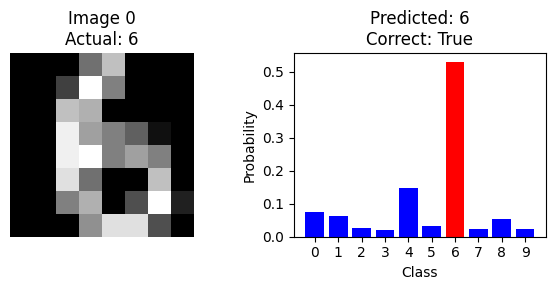
Can you find an image that is misclassified by the model?

Hint

The next code cell automatically finds examples of misclassified images, so try running it.

The code below identifies the first 5 misclassified images together with the model’s probability output:

# Get all predictions on the test set
Z1_test = W1 @ X_test + b1  # First layer pre-activation
H_test = np.maximum(0, Z1_test)  # ReLU activation
Z2_test = W2 @ H_test + b2  # Output layer logits
test_predictions = np.argmax(Z2_test, axis=0)  # Predicted classes
true_labels = np.argmax(Y_test, axis=0)  # True classes

# Find where the model makes mistakes
incorrect_indices = np.where(test_predictions != true_labels)[0]

# Display the first 5 misclassified images
plt.figure(figsize=(12, 8))

for i, idx in enumerate(incorrect_indices[:5]):
    # Show the image
    plt.subplot(2, 5, i+1)
    image_2d = X_test_orig[idx].reshape(8, 8)  # Reshape to 8x8
    plt.imshow(image_2d, cmap='gray')
    plt.title(f'Image {idx}\nTrue: {true_labels[idx]}\nPred: {test_predictions[idx]}')
    plt.axis('off')

    # Show probability distribution
    plt.subplot(2, 5, i+6)
    single_image = X_test[:, idx:idx+1]  # Get single image keeping shape
    Z1_single = W1 @ single_image + b1
    H_single = np.maximum(0, Z1_single)
    Z2_single = W2 @ H_single + b2
    probabilities = np.exp(Z2_single) / np.sum(np.exp(Z2_single))  # Softmax

    classes = range(10)
    # Color coding: red=true, green=predicted, blue=other
    colors = ['red' if c == true_labels[idx] else 
              ('green' if c == test_predictions[idx] else 'blue') 
              for c in classes]

    plt.bar(classes, probabilities.flatten(), color=colors)
    plt.xticks(classes)
    plt.xlabel('Class')
    plt.ylabel('Probability')

plt.tight_layout()
plt.show()

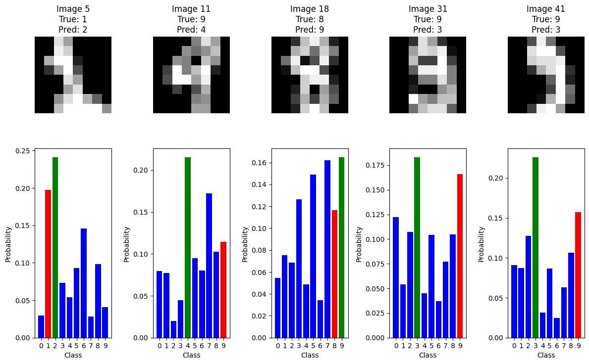
When you look at the misclassified examples and their probability distributions, what patterns do you notice? Try changing which misclassified images are shown and investigate whether these patterns are consistent.

Extra questions (optional)

1. Are you guaranteed to find the true minimum point of the loss function \(L\) using the gradient method above?

2. Why can you not simply find the minimum point of the loss function \(L\) directly? Can you plot the function \(L\) and visually read off the minimum?

3. The network function \(\Phi\) is determined by its weight matrices (\(W_1, W_2\)) and bias vectors (\(b_1, b_2\)). Compute the total number of these adjustable parameters in \(\Phi\)?

4. Can you mathematically verify the computation of some of the key gradients in the backward pass part of the code (e.g., dZ2 and dW2) in the for loop for epoch in range(100): in the Python code above?

9: Design of a Ring Detector

a: Problem statement

In this exercise, you will design and implement a deep neural network (with \(L=3\) layers) that can determine whether a point \((x_1,x_2)\) in the plane lies inside a circular ring (annulus). This is a classification problem where the network must be able to distinguish between points inside and outside the ring.

The mathematical definition of a circular ring is:

\[ \{(x_1,x_2) \in \mathbb{R}^2: a^2 \le x_1^2+x_2^2 \le b^2\}, \]

where \(a,b \in \mathbb{R}\).

A ReLU network creates decision boundaries that are piecewise linear. Since a circle is a curve, a simple ReLU network cannot represent it exactly.

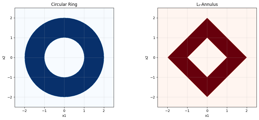
b: Approximation with an \(L_1\)-Annulus

To make the problem solvable with a simple network, we approximate the circular ring with a “diamond-shaped” ring, also known as an \(L_1\)-annulus. This shape has linear edges and is therefore perfectly suited to a ReLU network.

We will now design a network that precisely determines whether a point \((x_1,x_2)\) lies in the region:

\[\begin{equation*} \{(x_1,x_2):\ a \le |x_1| + |x_2| \le b\},\quad\text{with } a=1,\ b=2. \end{equation*}\]

A single linear layer cannot “cut a hole” in the middle, so the exercise requires a non-linear approach. We will use ReLU activations to construct the necessary absolute values and piecewise functions.

The code cell below visualizes the circular ring and the \(L_1\)-annulus that we consider:

# Grid
x1 = np.linspace(-2.5, 2.5, 500)
x2 = np.linspace(-2.5, 2.5, 500)
X1, X2 = np.meshgrid(x1, x2)

# Circular ring (a=1, b=2)
R = np.sqrt(X1**2 + X2**2)
ring_region = (R >= 1) & (R <= 2)

# L1-annulus (a=1, b=2)
L1_radius = np.abs(X1) + np.abs(X2)
L1_region = (L1_radius >= 1) & (L1_radius <= 2)

# Visualization
fig, (ax1, ax2) = plt.subplots(1, 2, figsize=(12, 5))

# Left plot: Circular ring
ax1.imshow(ring_region, extent=[-2.5, 2.5, -2.5, 2.5], origin='lower', cmap='Blues')
ax1.set_title('Circular Ring')
ax1.set_xlabel('x1')
ax1.set_ylabel('x2')
ax1.grid(True, alpha=0.3)

# Right plot: L1-annulus
ax2.imshow(L1_region, extent=[-2.5, 2.5, -2.5, 2.5], origin='lower', cmap='Reds')
ax2.set_title('L₁-Annulus')
ax2.set_xlabel('x1')
ax2.set_ylabel('x2')
ax2.grid(True, alpha=0.3)

plt.tight_layout()
plt.show()

c: Network architecture

We construct a deep neural ReLU network of the form \(2\to 4\to 3\to 1\).

State the sizes of the weight matrices \(W_1, W_2, W_3\) and the bias vectors \(b_1, b_2, b_3\). Verify that the network has 31 parameters in total.

Layer 1: Construction of \(|x_1|\) and \(|x_2|\)

The first layer computes the positive and negative parts of \(x_1\) and \(x_2\):

\[ h^{(1)}=\mathrm{ReLU}(W_1 X + b_1) \]

What should \(W_1\) and \(b_1\) be to produce the output

\[ h^{(1)}=[\mathrm{ReLU}(x_1),\ \mathrm{ReLU}(-x_1),\ \mathrm{ReLU}(x_2),\ \mathrm{ReLU}(-x_2)]^\top? \]

Answer

\[\begin{equation*} W_1=\begin{bmatrix} 1 & 0\\ -1 & 0\\ 0 & 1\\ 0 & -1 \end{bmatrix},\quad b_1=\begin{bmatrix}0\\0\\0\\0\end{bmatrix}. \end{equation*}\]

How can we express \(|x_1|\) and \(|x_2|\) using \(h^{(1)}\)?

Answer

We can express the absolute values as follows: \(|x_1|=h_1^{(1)}+h_2^{(1)}\) and \(|x_2|=h_3^{(1)}+h_4^{(1)}\).

The total \(L_1\) radius is therefore \(r=|x_1|+|x_2|=\sum_{i=1}^4 h_i^{(1)}\).

Layer 2: Computing distances to the boundaries

This layer computes the piecewise functions needed to determine whether \(r := |x_1| + |x_2|\) is between \(a=1\) and \(b=2\).

\[\begin{equation*} h^{(2)}=\mathrm{ReLU}(W_2 h^{(1)} + b_2), \end{equation*}\]

With \(a=1,\ b=2\) we get

\[\begin{equation*} W_2=\begin{bmatrix} -2 & -2 & -2 & -2\\ -1 & -1 & -1 & -1\\ 1 & 1 & 1 & 1 \end{bmatrix},\quad b_2=\begin{bmatrix}3\\2\\-2\end{bmatrix}. \end{equation*}\]

These neurons produce:

• \(h_1^{(2)} = \mathrm{ReLU}(3-2r) = \mathrm{ReLU}((b-r)-(r-a))\)

• \(h_2^{(2)} = \mathrm{ReLU}(2-r) = \mathrm{ReLU}(b-r)\)

• \(h_3^{(2)} = \mathrm{ReLU}(r-2) = \mathrm{ReLU}(r-b)\)

Output layer (Linear, no activation)

The last layer combines these pieces into a final score.

\[\begin{equation*} z^{(3)} = W_3 h^{(2)} + b_3,\quad W_3=\begin{bmatrix}-1 & 1 & -1\end{bmatrix},\quad b_3=\begin{bmatrix}0\end{bmatrix}. \end{equation*}\]

That is, the output is \(z^{(3)} = h_2^{(2)} - h_3^{(2)} - h_1^{(2)}\).

Decision rule: We predict that the point is “in the ring” if and only if \(z^{(3)} \ge 0\). (Points exactly on the boundary yield \(z^{(3)}=0\).)

d: Implementing the network

We implement the network below and test it on the following points:

def relu(z): return np.maximum(0, z)

# Layer 1
W1 = np.array([[ 1., 0.], [-1., 0.], [ 0., 1.], [ 0.,-1.]])
b1 = np.zeros((4,1))

# Layer 2 (a=1, b=2)
W2 = np.array([[-2.,-2.,-2.,-2.], [-1.,-1.,-1.,-1.], [ 1., 1., 1., 1.]])
b2 = np.array([[ 3.],[ 2.],[-2.]])

# Output
W3 = np.array([[-1., 1., -1.]])
b3 = np.array([[0.]])

def ring_score(X):
    'Computes the final score for a point (x1,x2).'
    X = np.asarray(X, dtype=float).reshape(2,1)
    h1 = relu(W1 @ X + b1)
    h2 = relu(W2 @ h1 + b2)
    Z3  = W3 @ h2 + b3 
    return float(Z3.item())

def in_ring(X):
    'Returns True if the point is in the ring, otherwise False.'
    return ring_score(X) >= 0.0

# Tests
tests = [(0,0), (0.5,0.5), (1.1,0), (1,1), (1.5,0.2), (2,0), (2.1,0)]
results = {pt: in_ring(pt) for pt in tests}
print(results)

{(0, 0): False, (0.5, 0.5): True, (1.1, 0): True, (1, 1): True, (1.5, 0.2): True, (2, 0): True, (2.1, 0): False}

Verify that the network correctly classifies all test points with respect to the \(L_1\)-annulus (the diamond-shaped ring). What is the predicted score for points that lie exactly on the boundary (e.g., (1,1))?

Answer

Yes, all points are classified correctly according to the \(L_1\)-annulus. Points exactly on the boundary, such as (1,1) (where \(r=2\)) or (0.5, 0.5) (where \(r=1\)), yield a score of exactly 0 and are therefore classified as “in the ring” according to our rule (\(z^{(3)} \ge 0\)).

Remember that the original goal was to detect the circular ring. How does this network function as an approximation to that problem? Which points in the plane will be misclassified if we use this network to detect the circular ring? (Hint: Compare the two plots from section b).

Answer

The network functions as an approximation because the \(L_1\)-annulus resembles the circular ring. Misclassifications occur in the regions where the two figures do not overlap:

1. False positives: Points in the “corners” of the \(L_1\)-annulus (e.g., close to (1.5, 1.5)), which lie outside the circular ring, will be classified as being inside the ring.

2. False negatives: Points along the axes (e.g., close to (0.8, 0)), which lie inside the circular ring, will be classified as being outside the ring.

The approximation is best along the axes (\(x_1=0\) or \(x_2=0\)) and worst along the diagonals (\(|x_1| = |x_2|\)).

Modify the network to work with an annulus with \(a=0.5\) and \(b=1.5\).
What needs to be changed in the network parameters?
Implement the modified version and test it on relevant points.

We have chosen \(a\) and \(b\) the same in the circular ring and the approximating diamond-shaped ring. Is this the best way to approximate a circular annulus with a diamond-shaped annulus?