import matplotlib
if not hasattr(matplotlib.RcParams, "_get"):
    matplotlib.RcParams._get = dict.get
Singular Value Decomposition (SVD)#
Introduction to SVD#
Singular Value Decomposition (SVD) of real matrices is based on the following theorem:
Any real \(m \times n\) matrix \(A\) can be written in SVD form
where \(V\) is an orthogonal \(n\times n\) matrix, \(\Sigma\) is an \(m\times n\) diagonal matrix, and \(U\) is an orthogonal \(m\times m\) matrix. The elements in \(\Sigma\) are called singular values, they are all \(\geq 0\) and are in non-increasing order.
In the first part of the project, we thoroughly examine \(2\times 2\) matrices with full rank. Note that for the SVD of a \(2\times 2\) matrix, only \(2\times 2\) matrices are involved. Here is an example of the SVD of a \(2\times 2\) matrix:
Setup#
We call the Python packages and procedures we need below:
# Libraries
import numpy as np
from numpy.linalg import svd, matrix_rank

import matplotlib
if not hasattr(matplotlib.RcParams, "_get"):
    matplotlib.RcParams._get = dict.get
import matplotlib.pyplot as plt

from matplotlib.patches import Circle
from matplotlib.colors import ListedColormap, BoundaryNorm
from matplotlib.image import imread
from ipywidgets import interact, FloatSlider, Layout
from IPython.display import clear_output
from PIL import Image
from scipy.optimize import brentq

# Display settings
np.set_printoptions(precision=3, suppress=True)
plt.rcParams.update({'figure.max_open_warning': 0})
Existence of Solutions#
Let \(A\) be a real 2x2 matrix with full rank. We will show an important result on the way to SVD: There exists an orthonormal basis \(\,(\boldsymbol{v_1},\boldsymbol{v_2})\,\) for \(\Bbb R^2\) such that the basis vectors’ images \(\,A\boldsymbol{v_1}\,\) and \(\,A\boldsymbol{v_2}\,\) are orthogonal.
For arbitrary \(\,t\in\Bbb R\,\) we consider the vectors
Show that \(\,\boldsymbol{x_1(t)}\,\) and \(\,\boldsymbol{x_2(t)}\,\) are orthogonal for all \(t.\)
Show that there exists a \(\,t_0\in \left[0,\frac {\pi}2\right]\) that makes the image vectors \(\, \boldsymbol{y_1(t_0)} = A\,\boldsymbol{x_1(t_0)}\,\) and \(\,\boldsymbol{y_2(t_0)} = A \,\boldsymbol{x_2(t_0)}\,\) orthogonal. Hint: Show that the function \(\,s(t)=\boldsymbol{y_1(t)}\cdot \boldsymbol{y_2(t)}\,\) is continuous, consider its value at the interval endpoints, and use Bolzano’s theorem.
With the number \(t_0\) and the function \(\,s(t)\,\) from the previous question: Show that \(\,s(t_0+ \frac{\pi}{2})=0\,.\) Hint: Exploit that for all \(t\) we have \(\,\cos(t+\frac{\pi}{2})=-\sin(t)\,\) and \(\,\sin(t+\frac{\pi}{2})=\cos(t)\,.\)
Explain that we have thus solved the problem.
Geometric Solution of SVD for 2x2 Matrix with Full Rank#
We establish here a procedure “unit_circle_ellipse” which visualizes the transformation of the unit circle by a given 2x2 matrix \(\,A\,:\)
def unit_circle_ellipse(A, slider_width='80%', figsize=(14, 7)):
    """
    Creates an interactive visualization of the unit circle and its image under matrix A.
    Parameters:
    - A: 2x2 numpy array, transformation matrix
    - slider_width: slider width (e.g., '80%')
    - figsize: tuple with figure size (width, height)
    """
    # Basis and image functions
    def x1(t): return np.array([np.cos(t), np.sin(t)])
    def x2(t): return np.array([-np.sin(t), np.cos(t)])
    def y1(t): return A @ x1(t)
    def y2(t): return A @ x2(t)

    # Precompute ellipse points
    ts = np.linspace(0, 2*np.pi, 361)
    ellipse_pts = np.column_stack([A @ x1(tt) for tt in ts]).T

    # Plot function
    def plot_vectors(t):
        clear_output(wait=True)
        fig, (ax1, ax2) = plt.subplots(1, 2, figsize=figsize)
        for ax in (ax1, ax2):
            ax.set_aspect('equal')
            ax.grid(True, linestyle='--', linewidth=0.4, alpha=0.5)
        # Common axis limits
        all_pts = np.vstack([ellipse_pts, x1(t), x2(t), y1(t), y2(t)])
        lim = 1.15 * np.max(np.abs(all_pts))
        for ax in (ax1, ax2):
            ax.set_xlim(-lim, lim)
            ax.set_ylim(-lim, lim)

        # Left: unit circle
        circle = Circle((0, 0), radius=1, edgecolor='lightgrey', facecolor='none', linewidth=1.5, zorder=0)
        ax1.add_patch(circle)
        ax1.plot(np.cos(ts), np.sin(ts), color='lightgrey', linewidth=1.5, zorder=0)
        # Right: ellipse
        ax2.plot(ellipse_pts[:, 0], ellipse_pts[:, 1], color='lightgrey', linewidth=1.5, zorder=0)

        # Function for arrows and labels
        def draw_arrow(ax, v, color, label, z):
            ax.quiver(0, 0, v[0], v[1], angles='xy', scale_units='xy', scale=1,
                      color=color, width=0.012, zorder=z)
            ax.text(v[0], v[1], f'  {label}{tuple(np.round(v, 2))}',
                    va='bottom', ha='left', fontsize=9, color=color)

        # Draw vectors
        draw_arrow(ax1, x1(t), 'tab:blue', 'x₁', 3)
        draw_arrow(ax1, x2(t), 'tab:blue', 'x₂', 3)
        draw_arrow(ax2, y1(t), 'tab:red',  'y₁', 4)
        draw_arrow(ax2, y2(t), 'tab:red',  'y₂', 4)

        ax1.set_title('The Unit Circle S')
        ax2.set_title('The Ellipse A.S')
        fig.suptitle(rf"$t={t:.2f}$   (drag the slider)", fontsize=14)
        plt.show()

    # Slider
    slider = FloatSlider(
        value=0,
        min=0,
        max=2*np.pi,
        step=0.01,
        description='t',
        continuous_update=True,
        readout_format='.2f',
        layout=Layout(width=slider_width)
    )
    interact(plot_vectors, t=slider)
In the following cell you should enter the matrix you want to test. Try \(\,A=\left[\begin{array}{c}1 & 2\\-1 & 1\end{array}\right]\,\) for graphical solution with slider.
Run the cell, so the procedure
unit_circle_ellipseis activated.
A = np.array([[1,2],
              [-1,1]])
unit_circle_ellipse(A)
We proceed based on the situation and the terms as in exercise 1. Proceed as follows:
Find with the slider a \(\,t_0,\,\) such that \(\,\boldsymbol{y_1(t_0)}\,\) and \(\,\boldsymbol{y_2(t_0)}\,\) are orthogonal.
Set \(\,\boldsymbol{v_1}=\boldsymbol{x_1(t_0)}\,\) and \(\,\boldsymbol{v_2}=\boldsymbol{x_2(t_0)}\,\)
Let \(\sigma_1\) and \(\sigma_2\) be the lengths \(\,\sigma_1=\left\|\boldsymbol{y_1(t_0)}\right\|\,\) and \(\,\sigma_2=\left\|\boldsymbol{y_2(t_0)}\right\|\,\)
Set \(\,\boldsymbol{u_1}=\frac{1}{\sigma_1}\,\boldsymbol{y_1(t_0)}\,\) and \(\,\boldsymbol{u_2}=\frac{1}{\sigma_2}\,\boldsymbol{y_2(t_0)}\,\)
Show that \(\,V=\left[\boldsymbol{v_1}\,\,\boldsymbol{v_2}\right]\,\) and \(\,U=\left[\boldsymbol{u_1}\,\,\boldsymbol{u_2}\right]\,\) are orthogonal matrices.
Let \(\Sigma\) be the diagonal matrix \(\,\Sigma=\begin{bmatrix}\sigma_1&0\\0&\sigma_2\end{bmatrix},\) and show that \(\,A\,V=U\,\Sigma\,\)
Show and verify in the given example that \(\,A=U\,\Sigma\,V^T\,\)
Convention: It is standard convention in SVD that one wants the singular values in decreasing order, that is, \(\,\sigma_1 \geq \sigma_2\,.\) Conveniently, in the first example we found a \(\,t_0\in \left[0,\frac {\pi}2\right],\,\) where \(\,\left\|\boldsymbol{y_1(t_0)}\right\|>\left\|\boldsymbol{y_2(t_0)}\right\|\,.\) If the opposite is true, simply move the slider to the next orthogonality point. This occurs at the \(\,t\)-angle \(\,t_0+\frac{\pi}2\,\) where the lengths are exchanged.
Try for example \(\,A=\left[\begin{array}{c}1 & -1\\0 & 2\end{array}\right]\,\) or \(\,A=\left[\begin{array}{c}1 & -1\\0 & -2\end{array}\right]\,.\)
Manual calculation version where you can work with exact numbers:
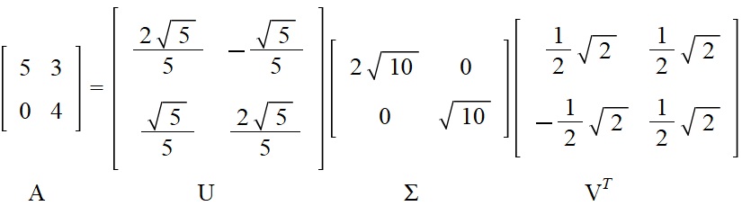
Perform SVD on \(\,A=\left[\begin{array}{c}5 & 3\\0 & 4\end{array}\right]\,.\)
We now establish a procedure SVD_2x2_matrix which collects points 1-7, and which you can use to test your 2x2 matrices:
Note in particular that we ensure that \(\,\|\boldsymbol{y_1(t_0)}\|\,\) is greater than or equal to \(\,\|\boldsymbol{y_2(t_0)}\|\,.\)
def SVD_2x2_matrix(A, print_output = False):

    # Basis vectors as a function of t
    def x1(t): return np.array([np.cos(t), np.sin(t)])
    def x2(t): return np.array([-np.sin(t), np.cos(t)])
    def y1(t): return A.dot(x1(t))
    def y2(t): return A.dot(x2(t))

    # Dot product function
    f = lambda t: np.dot(y1(t), y2(t))

    # Find root in (0, p/2)
    t0 = brentq(f, 1e-6, np.pi/2 - 1e-6)

    # Ensure ||y1|| >= ||y2||
    if np.linalg.norm(y1(t0)) < np.linalg.norm(y2(t0)):
        t0 += np.pi/2

    # Then we can set the values directly:
    sigma1 = np.linalg.norm(y1(t0))
    sigma2 = np.linalg.norm(y2(t0))
    Sigma = np.diag([sigma1, sigma2])
    V = np.column_stack([x1(t0), x2(t0)])
    U = np.column_stack([y1(t0)/sigma1, y2(t0)/sigma2])

    # print output if selected
    if print_output:
        print("t0 =", t0)
        print("S =\n", Sigma)
        print("V =\n", V)
        print("U =\n", U)

    return  t0, U, Sigma, V
In the following cell the procedure SVD_2x2_matrix is tested. As output you get in this order: \(\,t_0,\, U, \,\Sigma\,\) and \(\,V\,.\)
Enter your test matrix \(A\) and check in a following cell that we achieve the desired decomposition \(\,A = U\, \Sigma\,V^T\,.\)
A = np.array([[1,2],
              [-1,1]])
t0, U, Sigma, V = SVD_2x2_matrix(A, print_output=True)
t0 = 1.2767950250213542
S =
 [[2.303 0.   ]
 [0.    1.303]]
V =
 [[ 0.29  -0.957]
 [ 0.957  0.29 ]]
U =
 [[ 0.957 -0.29 ]
 [ 0.29   0.957]]
Testing Special Matrices#
Create simple test examples of special 2x2 matrices:
Symmetric matrix, i.e., the type \(\,\left[\begin{array}{c}a & b\\b & c\end{array}\right]\)
Skew-symmetric matrix of the type \(\,\left[\begin{array}{c}a & b\\-b & a\end{array}\right]\)
Orthogonal matrix (you can for example use matrix \(U\) stored from the previous exercise)
The test matrices are written in the following cell. When you run the cell, you activate both procedures unit_circle_ellipse and SVD_2x2_matrix.
Experiment using the slider and study the algebraic output on matrices of type 1-3. Discuss what is special!
A = np.array([[1,2],
              [-1,1]])
unit_circle_ellipse(A)
_ = SVD_2x2_matrix(A, print_output=True)
t0 = 1.2767950250213542
S =
 [[2.303 0.   ]
 [0.    1.303]]
V =
 [[ 0.29  -0.957]
 [ 0.957  0.29 ]]
U =
 [[ 0.957 -0.29 ]
 [ 0.29   0.957]]
Gilbert Strang’s Visualization of SVD#
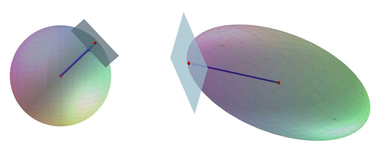
The world’s most well-known teacher of linear algebra, Gilbert Strang from MIT, is asked in a 5-minute YouTube interview what is most beautiful in linear algebra, and his answer is SVD. When asked what is beautiful in SVD, he answers that every matrix can be viewed as a rotation followed by stretching in orthogonal directions and concluded with another rotation. Since rotations do not change the shape of a geometric object, it is the middle part, the stretches, that is the crucial part. And they are given by the singular values. We will now study this more closely via a figure from an article by Gilbert Strang:
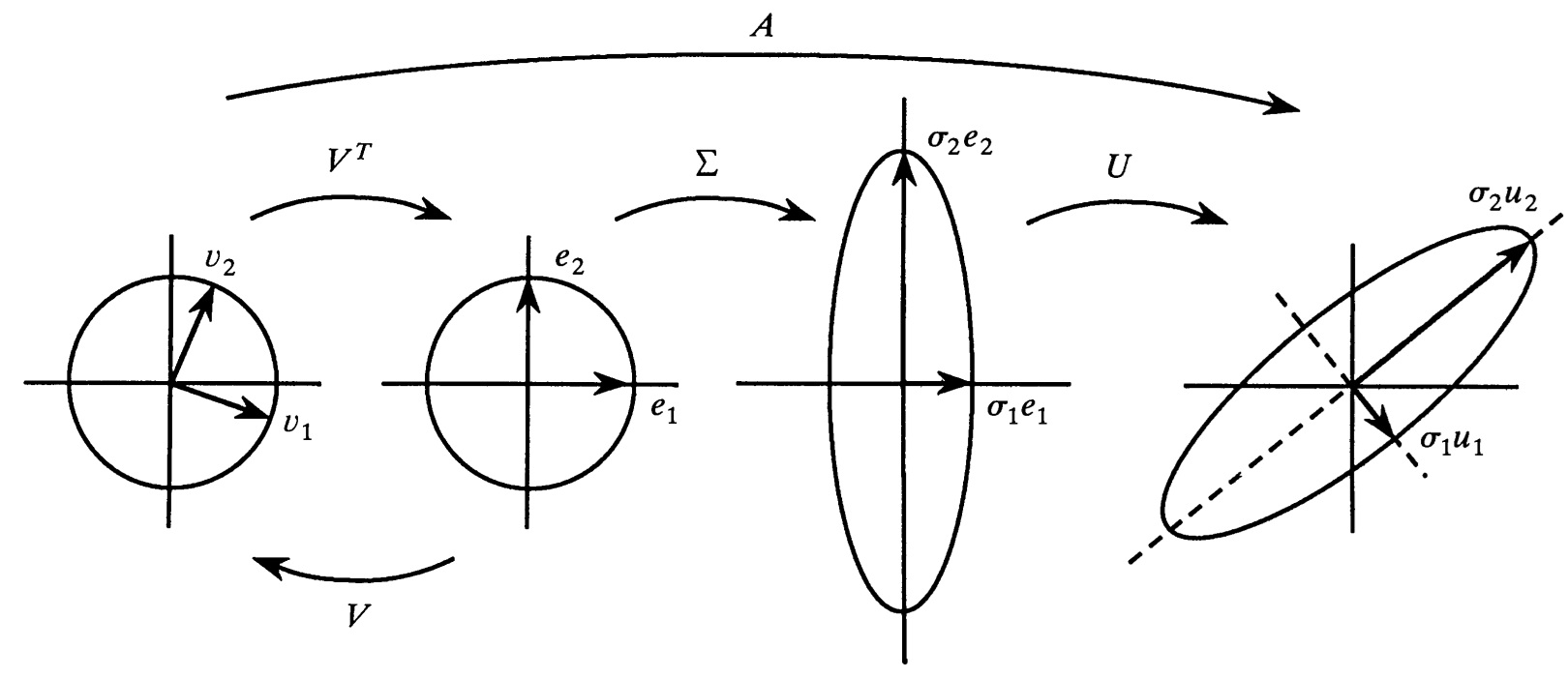
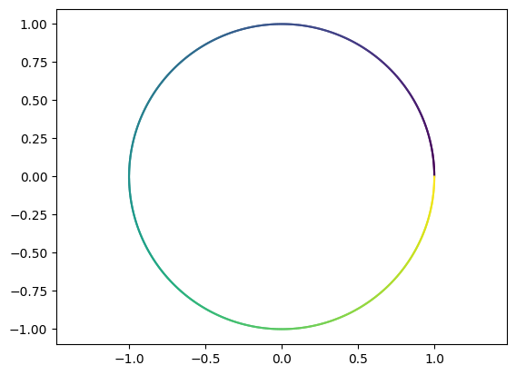
Instead of looking at the transformation of the unit circle all at once, as we would by going directly from the left side to the right side in the figure, we capture it in three steps determined by the right-hand side of the SVD \(\,A=U\,\Sigma\,V^T\,.\) Before we start, we recall that an ellipse can be thought of as a circle that has been stretched in two orthogonal directions. In standard parametric form, the ellipse \(e\) is therefore given by \(\,e(t)=\big (a\cos(t),b\sin(t)\big )\,,\,\,t\in [0,2\pi]\,\) where \(a\) and \(b\) are the stretch factors, also called semi-axes.
Here is an example you can work with:
The transformation of the unit circle \(C\) is naturally independent of which parametrization we choose for it. We therefore choose, inspired by the Gilbert Strang figure, the standard parametrization for \(c_v\) in the new coordinate system determined by the basis vectors \(\boldsymbol{y_1(t_0)}\) and \(\boldsymbol{y_2(t_0)}\) (i.e., the columns of \(V\)).
The exercises in this section are think exercises. Ready-to-run implementations that plot the relevant parametrizations are provided.
What parametrization \(c_e\) does \(C\) then have in the standard coordinate system determined by the basis vectors \(\boldsymbol{v_1}\) and \(\boldsymbol{x_1(t_0)}\,?\)
Hint: \(V\) is the change of basis matrix that converts \(v\)-coordinates to standard \(e\)-coordinates.
def plot_parametric(func):
"""
Plots a parametric curve defined by func(t) for t in [0, 2p],
with a color gradient along the path.
Parameters:
- func: lambda function of t, returning (x, y)
"""
N = 500
t = np.linspace(0, 2*np.pi, N)
x, y = func(t)
# Normalize t for colormap
colors = plt.get_cmap("viridis")(np.linspace(0, 1, N))
for i in range(N-1):
plt.plot(x[i:i+2], y[i:i+2], color=colors[i])
plt.axis("equal")
plt.show()
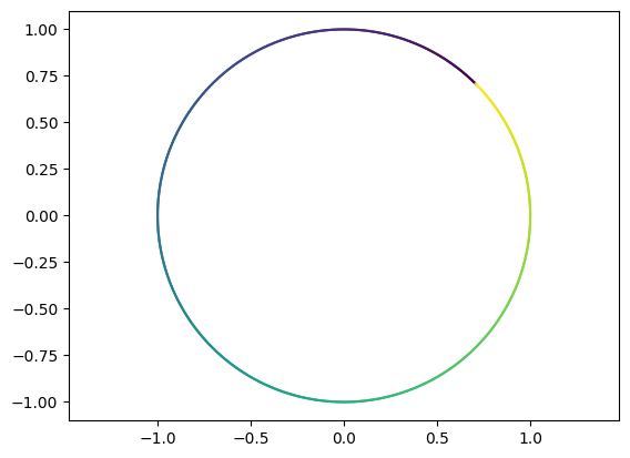
V = np.array([[1,-1],
[1, 1]]) * np.sqrt(2)/2
cv = lambda t: np.array([np.cos(t), np.sin(t)]) # function for standard parametrization of unit circle in v basis
ce = lambda t: V @ cv(t) # unit circle in standard basis
plot_parametric(ce)
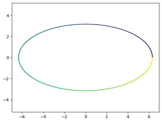
Perform the first transformation \(V^T\,c_e\). Comment on the result.
# first transformation
T1 = lambda t: V.T @ ce(t)
plot_parametric(T1)
Perform the next transformation \(\,\Sigma\,(V^T\,c_e)\,.\) What geometric figure are we dealing with?
Sigma = np.diag([2,1])*np.sqrt(10)

# second transformation
T2 = lambda t: Sigma @ T1(t)
plot_parametric(T2)
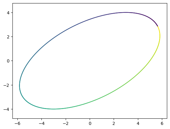
Can you already see why \(\,A\, c_e=U\,(\Sigma\,(V^T\,c_e))\,\) is an ellipse? What are its semi-axes?
The following cell shows the final image \(A\,C\).
A = np.array([[5,3],
              [0,4]])
plot_parametric(lambda t: A @ ce(t))
Geometric Solution for 3x3 Matrices: “Apollonius’ Method”#
A 3x3 matrix \(A\) with full rank is given by
The goal of the exercise is to find an SVD for \(A\). For this purpose, we introduce a linear map \(f: \mathbb{R}^3\to \mathbb{R}^3\) given by \(f(\boldsymbol{v})=A\, \boldsymbol{v}\) for all \(\boldsymbol{v}\) in \(\mathbb{R}^3\).
We wish to find the SVD of \(A\) by examining how \(f\) transforms the unit sphere \(K = \{ (x,y,z) \in \mathbb{R}^3 \;\;|\;\; x^2 + y^2 + z^2 = 1 \}\). We denote the image \(f(K)\) by \(E\).
The following knowledge is available for the exercise:
A linear map given by a \(3\times 3\) matrix with full rank preserves tangent planes. This means that the tangent plane for \(K\) at a point \(P\) on \(K\) is mapped to the tangent plane for \(E\) at \(f(P)\).
There are 6 points on \(E\) where the position vector of each point is orthogonal to the tangent plane for \(E\) at that point.
The 6 points occur in 3 pairs of opposite points.
If you choose one point from each of the three pairs, the three points’ position vectors will be mutually orthogonal, and with them we can construct the SVD.
Question 1#
You need to find three points on \(E\) whose position vectors are mutually orthogonal. Let \(P=(x_0,y_0,z_0)\) be an arbitrary point on \(K\). Using the following procedure, we set up a nonlinear system of equations in \(x_0,y_0,z_0\), which we will solve using scipy’s fsolve, which can find the roots of a function numerically. It will be set up later in the exercise in the function equations_LS(P).
from scipy.optimize import fsolve
A = np.array([[1,2,1],
              [1,1,-1],
              [-1,0,0]])
Show that the tangent plane \(TK_P\) for \(K\) at \(P\) is given by
\[ x_0\cdot x+y_0\cdot y+z_0\cdot z=1\;. \]
Now assume that \(x_0\) is different from 0 and continue.
Show that the vectors
\[\begin{split} \boldsymbol{r}_1=\begin{bmatrix} -\frac{y_0}{x_0}\\1\\0\end{bmatrix}\quad \text{ and }\quad\boldsymbol{r}_2=\begin{bmatrix} -\frac{z_0}{x_0}\\0\\1\end{bmatrix} \end{split}\]are linearly independent direction vectors for \(TK_P\).
Hint: Find a parametric representation for \(TK_P\).
In the following cell we define a function that returns \(\boldsymbol{r}_1\) and \(\boldsymbol{r}_2\) given \(P\). This is a helper function that will be used later.
def TK_vectors(P):
    """Returns two linearly independent direction vectors for the tangent plane to K at point P"""
    x0, y0, z0 = P
    r1 = np.array([-y0/x0, 1, 0])
    r2 = np.array([-z0/x0, 0, 1])
    return r1, r2
Let \(Q\) be the image point \(Q=f(P)\) (Q=A@P), and let \(TE_Q\) be the tangent plane for \(E\) at \(Q\).
Specify two linearly independent direction vectors \(\boldsymbol{s}_1\) and \(\boldsymbol{s}_2\) for \(TE_Q\). Hint: Consider again the parametric representation for \(TK_P\).
In the following cell we define another helper function that returns \(\boldsymbol{s}_1\) and \(\boldsymbol{s}_2\) given point \(P\).
Complete the function. Hint: You may use the
TK_vectorsfunction from before.
def TE_vectors(P):
    """Returns two linearly independent direction vectors for the tangent plane to E at point Q=f(P)"""
    x0, y0, z0 = P
    r1, r2 = TK_vectors(P)
    # YOUR CODE: Define s1 and s2

    return s1, s2
Can you justify that \(\boldsymbol{s}_1\) and \(\boldsymbol{s}_2\) are actually linearly independent?
With this, we have that \(TE_Q\) can be parametrized as \(Q+t_1\boldsymbol{s}_1+t_2\boldsymbol{s}_2\).
Show that the position vector \(OQ\) of \(Q\) is orthogonal to \(TE_Q\) precisely when the following 3 equations are satisfied.
\(\quad OQ \cdot \boldsymbol{s}_1 = 0\)
\(\quad OQ \cdot \boldsymbol{s}_2 = 0\)
\(\quad x_0^2 + y_0^2 + z_0^2 - 1 = 0\)
\(OQ\) is determined from \(P\) through the mapping \(f\), and \(\boldsymbol{s}_1\) and \(\boldsymbol{s}_2\) are determined correspondingly from \(P\) as shown in TE_vectors. Thus all three equations in the system of equations depend only on the unknown \(P=(x_0,y_0,z_0)\).
In the following cell we define a function that computes the left-hand sides of the 3 equations above. This is the function whose root we want to find, since all right-hand sides are 0.
Complete the function. Hint: You may use
Numpy’s functionsnp.dot(v,w),np.linalg.norm(v). In Python, \(x^a\) is written asx**a.
def equations_LS(P):
    """Returns the values of the left-hand sides of the three equations in the nonlinear system of equations"""
    x0, y0, z0 = P
    Q = A @ P
    s1, s2 = TE_vectors(P)
    # define the values of the left-hand sides of the system of equations
    eq1_LS =
    eq2_LS =
    eq3_LS =
    return (eq1_LS, eq2_LS, eq3_LS)
  Cell In[14], line 7
    eq1_LS =
            ^
SyntaxError: invalid syntax
In the following cell we find the roots of the system of equations using fsolve. fsolve takes a function and an initial guess as input. We therefore also define random initial guesses on \(K\). The solutions found are thus also points \((x_0,y_0,z_0)\) on \(K\).
Run the cell.
solutions = [] # list of solutions

# different initial guesses for fsolve
guesses = [np.random.normal(size=3) for _ in range(50)] # 50 random guesses
guesses = [g/np.linalg.norm(g) for g in guesses] # normalizes guesses so they lie on K

# find solutions for each initial guess
for guess in guesses:
    # avoid x0 close to 0 (the assumption!) - skip the initial guess
    if abs(guess[0]) <= 0.05:
        continue

    # find solution with fsolve
    sol = fsolve(equations_LS, guess)

    # check if solution is new (not already found)
    if not any(np.allclose(sol, s) for s in solutions):
        # save the solution
        solutions.append(sol)

# print the solutions
i = 0
for solution in solutions:
    print(f'solutions[{i}] =', solution)
    i += 1
---------------------------------------------------------------------------
NameError                                 Traceback (most recent call last)
Cell In[15], line 14
     11     continue
     13 # find solution with fsolve
---> 14 sol = fsolve(equations_LS, guess)
     16 # check if solution is new (not already found)
     17 if not any(np.allclose(sol, s) for s in solutions):
     18     # save the solution

NameError: name 'equations_LS' is not defined
Verify that 6 solutions have been found.
If not, you may have been unlucky with the random initial guesses, or we may have made an error about the assumption that \(x_0\) is different from 0. Revisit the investigation for the case \(x_0=0\) and find the remaining solutions.
If 6 solutions have been found, then show that Question 1 is answered.
Question 2#
Determine an SVD for \(A\). We need to find three \(3\times 3\) matrices \(\Sigma\), \(V\), and \(U\), where \(\Sigma\) is a diagonal matrix, and \(V\) and \(U\) are orthogonal.
Proceed according to the following procedure.
Using your found solutions to
equations_LS, select 3 points on \(E\) whose position vectors are mutually orthogonal, and determine the lengths of the three vectors. Hint: You may usenp.linalg.norm(v).
e1 = A @ solutions[]
e2 = A @ solutions[]
e3 = A @ solutions[]
print("e1 =", e1, "with length", np.linalg.norm(e1))
print("e2 =", e2, "with length", np.linalg.norm(e2))
print("e3 =", e3, "with length", np.linalg.norm(e3))
  Cell In[16], line 1
    e1 = A @ solutions[]
                       ^
SyntaxError: invalid syntax
Arrange the three lengths in non-increasing order and call them \(\sigma_1\), \(\sigma_2\), and \(\sigma_3\). Form the diagonal matrix \(\Sigma\). Hint: You may use
np.diag([a,b,c]).
sigma1 = np.linalg.norm()
sigma2 = np.linalg.norm()
sigma3 = np.linalg.norm()
Sigma = np.diag([sigma1, sigma2, sigma3])
print("Sigma =\n", Sigma)
---------------------------------------------------------------------------
TypeError                                 Traceback (most recent call last)
Cell In[17], line 1
----> 1 sigma1 = np.linalg.norm()
      2 sigma2 = np.linalg.norm()
      3 sigma3 = np.linalg.norm()

TypeError: norm() missing 1 required positional argument: 'x'
Find the three position vectors for points on \(K\) whose images have lengths \(\sigma_1\), \(\sigma_2\), and \(\sigma_3\), and call them \(\boldsymbol{v}_1\), \(\boldsymbol{v}_2\), and \(\boldsymbol{v_3}\), respectively. Form the matrix \(V\).
Hint: You may usenp.column_stack([u,v,w]).
v1 = solutions[]
v2 = solutions[]
v3 = solutions[]
V = np.column_stack([v1, v2, v3])
print("V =\n", V)
  Cell In[18], line 1
    v1 = solutions[]
                   ^
SyntaxError: invalid syntax
Determine the vectors \(\boldsymbol{u}_1=\frac{1}{\sigma_1}f(\boldsymbol{v}_1)\), \(\boldsymbol{u}_2=\frac{1}{\sigma_2}f(\boldsymbol{v}_2)\), and \(\boldsymbol{u}_3=\frac{1}{\sigma_3}f(\boldsymbol{v}_3)\). Form the matrix \(U\).
u1 = (1/sigma1) * (A @ v1)
u2 = (1/sigma2) * (A @ v2)
u3 = (1/sigma3) * (A @ v3)
U = np.column_stack([u1, u2, u3])
print("U =\n", U)
---------------------------------------------------------------------------
NameError                                 Traceback (most recent call last)
Cell In[19], line 1
----> 1 u1 = (1/sigma1) * (A @ v1)
      2 u2 = (1/sigma2) * (A @ v2)
      3 u3 = (1/sigma3) * (A @ v3)

NameError: name 'sigma1' is not defined
Verify that \(A=U\,\Sigma\,V^T\).
print("A =\n",A)
print("U@Sigma@V.T =\n",U @ Sigma @ V.T)
A =
 [[ 1  2  1]
 [ 1  1 -1]
 [-1  0  0]]
U@Sigma@V.T =
 [[ 4.928  3.632]
 [-0.844  3.436]]
Matrix Approximation#
SVD command for an \(m\times n\) matrix \(A\)#
An \(m\times n\) matrix with random integers between, for example, \(1\) and \(5\) as entries can be created with np.random.randint().
Choose \(m\) and \(n\) and create a randomly generated matrix
m = 'INSERT CODE HERE'
n = 'INSERT CODE HERE'
np.random.seed(0) # locks in the randomness
A = np.random.randint(1,6,size=(m,n))
A
---------------------------------------------------------------------------
UFuncTypeError                            Traceback (most recent call last)
Cell In[21], line 4
      2 n = 'INSERT CODE HERE'
      3 np.random.seed(0) # locks in the randomness
----> 4 A = np.random.randint(1,6,size=(m,n))
      5 A

File numpy/random/mtrand.pyx:782, in numpy.random.mtrand.RandomState.randint()

File numpy/random/_bounded_integers.pyx:1315, in numpy.random._bounded_integers._rand_int64()

File /builds/ctm/ctmweb/venv/lib/python3.11/site-packages/numpy/core/fromnumeric.py:3100, in prod(a, axis, dtype, out, keepdims, initial, where)
   2979 @array_function_dispatch(_prod_dispatcher)
   2980 def prod(a, axis=None, dtype=None, out=None, keepdims=np._NoValue,
   2981          initial=np._NoValue, where=np._NoValue):
   2982     """
   2983     Return the product of array elements over a given axis.
   2984
   (...)   3098     10
   3099     """
-> 3100     return _wrapreduction(a, np.multiply, 'prod', axis, dtype, out,
   3101                           keepdims=keepdims, initial=initial, where=where)

File /builds/ctm/ctmweb/venv/lib/python3.11/site-packages/numpy/core/fromnumeric.py:88, in _wrapreduction(obj, ufunc, method, axis, dtype, out, **kwargs)
     85         else:
     86             return reduction(axis=axis, out=out, **passkwargs)
---> 88 return ufunc.reduce(obj, axis, dtype, out, **passkwargs)

UFuncTypeError: ufunc 'multiply' did not contain a loop with signature matching types (dtype('<U16'), dtype('<U16')) -> None
The SVD command np.linalg.svd(A) for a matrix \(A\) gives the (\(m\times m\))-matrix \(U\), the (\(n\times n\))-matrix \(V^T\) and a vector \(\boldsymbol{s}\) with singular values in non-increasing order.
Use the SVD command to obtain \(U\), \(V^T\) and the vector \(\boldsymbol{s}\) for the matrix \(A\).
# Calculate SVD
U, s, Vt = 'INSERT CODE HERE'
print('\nSingular values (s):', s)
print('\nU =\n', U)
print('\nVt =\n', Vt)
---------------------------------------------------------------------------
ValueError                                Traceback (most recent call last)
Cell In[22], line 2
      1 # Calculate SVD
----> 2 U, s, Vt = 'INSERT CODE HERE'
      3 print('\nSingular values (s):', s)
      4 print('\nU =\n', U)

ValueError: too many values to unpack (expected 3)
Create the \(\Sigma\) matrix from the singular values in \(\boldsymbol{s}\) by completing the code below.
# We create a zero matrix with the same dimensions as A (m x n).
Sigma = np.zeros((m, n))

# Insert the singular values (s) on the diagonal.
for i in range(min(m, n)):
    Sigma[i, i] = 'INSERT CODE HERE'

print('\nSigma =\n', Sigma)
---------------------------------------------------------------------------
TypeError                                 Traceback (most recent call last)
Cell In[23], line 2
      1 # We create a zero matrix with the same dimensions as A (m x n).
----> 2 Sigma = np.zeros((m, n))
      4 # Insert the singular values (s) on the diagonal.
      5 for i in range(min(m, n)):

TypeError: 'str' object cannot be interpreted as an integer
Show that the SVD command matches by forming the product \(U\Sigma V^T\).
# Remember to use @ for matrix multiplication
recon = 'INSERT CODE HERE'
print('\nReconstruction (U @ Sigma @ Vt) =\n', np.round(recon,3))
print('\nA =\n', A)
---------------------------------------------------------------------------
UFuncTypeError                            Traceback (most recent call last)
Cell In[24], line 3
      1 # Remember to use @ for matrix multiplication
      2 recon = 'INSERT CODE HERE'
----> 3 print('\nReconstruction (U @ Sigma @ Vt) =\n', np.round(recon,3))
      4 print('\nA =\n', A)

File /builds/ctm/ctmweb/venv/lib/python3.11/site-packages/numpy/core/fromnumeric.py:3360, in round(a, decimals, out)
   3269 @array_function_dispatch(_round_dispatcher)
   3270 def round(a, decimals=0, out=None):
   3271     """
   3272     Evenly round to the given number of decimals.
   3273
   (...)   3358
   3359     """
-> 3360     return _wrapfunc(a, 'round', decimals=decimals, out=out)

File /builds/ctm/ctmweb/venv/lib/python3.11/site-packages/numpy/core/fromnumeric.py:56, in _wrapfunc(obj, method, *args, **kwds)
     54 bound = getattr(obj, method, None)
     55 if bound is None:
---> 56     return _wrapit(obj, method, *args, **kwds)
     58 try:
     59     return bound(*args, **kwds)

File /builds/ctm/ctmweb/venv/lib/python3.11/site-packages/numpy/core/fromnumeric.py:45, in _wrapit(obj, method, *args, **kwds)
     43 except AttributeError:
     44     wrap = None
---> 45 result = getattr(asarray(obj), method)(*args, **kwds)
     46 if wrap:
     47     if not isinstance(result, mu.ndarray):

UFuncTypeError: ufunc 'multiply' did not contain a loop with signature matching types (dtype('<U16'), dtype('float64')) -> None
A rank-\(r\) matrix is a sum of \(r\) linearly independent rank-\(1\) matrices#
Let \(A\) be an \(m \times n\) matrix with rank \(r \leq \min\{m,n\}\) and let \(\boldsymbol{u_1}, \boldsymbol{u_2}, \dots, \boldsymbol{u_r}\) denote the first \(r\) columns in \(U\) and \(\boldsymbol{v_1}^T, \boldsymbol{v_2}^T, \dots, \boldsymbol{v_r}^T\) the first \(r\) rows in \(V^T\).
The matrix \(A\) can then be written as the sum
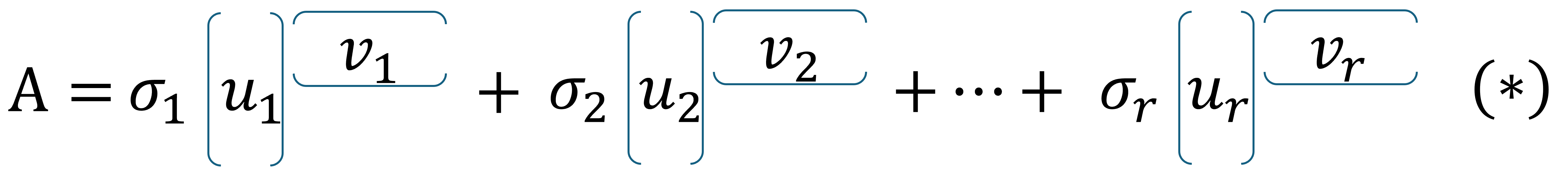
For large matrices with low rank, the above is an efficient storage method with minimal number consumption of numbers. We therefore introduce the term storage ratio \(SR\).
Show that \(SR\) is given by
\[ SR(r,m,n) = \dfrac{r (1 + m + n)}{m n} \]
Comment briefly on what happens to the storage ratio when \(r\) approaches \(\min(m, n)\).
We are looking at the matrix
\(A\) has the SVD decomposition
Determine the rank of \(A\) directly from the SVD arrangement.
Verify your answer by defining \(A\) using the command
np.array([], dtype=int)and use the commandnp.linalg.matrix_rank()to find the rank.
# DEFINE A HERE AND FIND THE RANK
Use \(\boldsymbol{u_1}\), \(\boldsymbol{u_2}\) and \(\boldsymbol{u_3}\) as well as \(\boldsymbol{v_1}^T\), \(\boldsymbol{v_2}^T\) and \(\boldsymbol{v_3}^T\) in the code cell below to verify \((*)\) in the example.
You can usenp.outer()to calculate \(\boldsymbol{u_i}\boldsymbol{v_i}^T\).
# Singular vectors from SVD (as shown earlier)
u1 = np.array([1/2, 1/2, 1/2, 1/2])
u2 = np.array([1/2, -1/2, -1/2, 1/2])
u3 = np.array([1/2, -1/2, 1/2, -1/2])

v1T = np.array([2/3, -1/3, 2/3])
v2T = np.array([2/3, 2/3, -1/3])
v3T = np.array([-1/3, 2/3, 2/3])

# Singular values
sigma1, sigma2, sigma3 = 24, 12, 6

# Verify the relation (*)
A_reconstructed = 'INSERT CODE HERE'

print("A reconstructed from u1,u2,u3 and v1T,v2T,v3T:\n", A_reconstructed)
A reconstructed from u1,u2,u3 and v1T,v2T,v3T:
 INSERT CODE HERE
The function below calculates the storage ratio \(SR\) given \(r\), \(m\), and \(n\).
def storage_ratio(r, m, n):
    return r*(1+m+n)/(m*n)
Determine the storage ratio for \(A\) by using the function
storage_ratio.
# INSERT CODE HERE
NB: For small matrices with high rank, \((*)\) is an expensive way to store!
Rank-\(k\) matrix approximation and retained information#
Given an \(m \times n\) matrix \(A\) with rank \(r \leq \min\{m,n\}\) and let \(k\) be a positive integer with \(k \leq r\). A rank-\(k\) approximation \(A_k\) of \(A\) is obtained by truncating the full SVD for \(A\), that is, by only keeping the first \(k\) singular values and corresponding singular vectors, while the remaining singular values are set to \(0\).
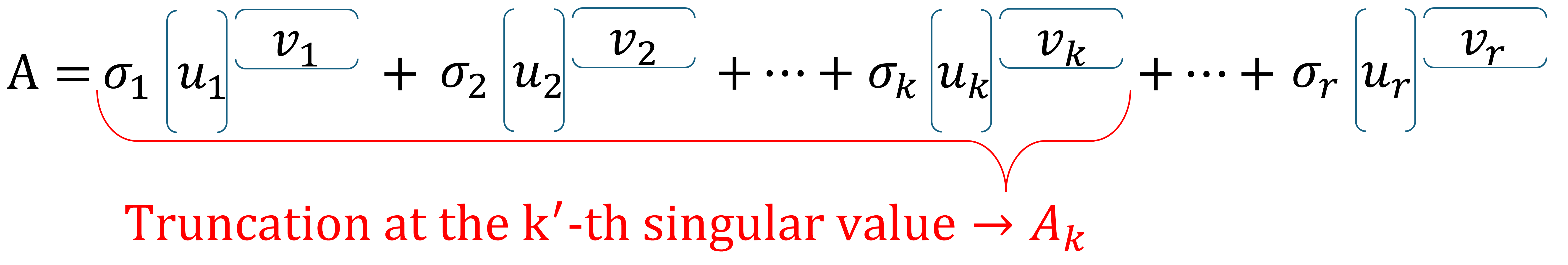
This can be written mathematically as:
We consider again the matrix
Husk at \(A\) har SVD-dekompositionen
Determine rank-\(1\), rank-\(2\), and rank-\(3\) approximations \(A_1\), \(A_2\), and \(A_3\) using \((*)\) below.
# Rank-1 approximation
A1 = 'INSERT CODE HERE'

# Rank-2 approximation
A2 = 'INSERT CODE HERE'

# Rank-3 approximation
A3 = 'INSERT CODE HERE'

# Print the results
print("Rank-1 approximation A1:\n", A1)
print("\nRank-2 approximation A2:\n", A2)
print("\nRank-3 approximation A3:\n", A3)
Rank-1 approximation A1:
 INSERT CODE HERE

Rank-2 approximation A2:
 INSERT CODE HERE

Rank-3 approximation A3:
 INSERT CODE HERE
How large is the difference between \(A\) and its approximations?
Define \(A\) in the code cell below and calculate \(A-A_1\), \(A-A_2\), and \(A-A_3\) and compare the three results.
# INSERT CODE HERE
How much information is retained through approximation?#
It is clear that the more singular values we include, the better the approximation becomes. We talk about how much information is retained through the approximation.
There are several ways to assess how much information is retained. The formula we use here depends only on how many singular values are included, which for rank-\(k\) approximation is \(k\) singular values.
The retained information \(RI\) for rank-\(k\) approximation of an \(m\times n\) matrix \(A\) with rank \(r\) is given by
where \(\sigma_1, \dots, \sigma_r\) are the non-negative singular values of \(A\), and \(r = \text{rank}(A)\).
Determine the retained information for approximations \(A_1\), \(A_2\), and \(A_3\) in our example.
# Rank of A
r = len(s)

# Retained information: k = 1,2,3
RI1 = 'INSERT CODE HERE'
RI2 = 'INSERT CODE HERE'
RI3 = 'INSERT CODE HERE'

print("Retained information for rank-1 approximation:", np.round(RI1,3))
print("Retained information for rank-2 approximation:", np.round(RI2,3))
print("Retained information for rank-3 approximation:", np.round(RI3,3))
---------------------------------------------------------------------------
NameError                                 Traceback (most recent call last)
Cell In[31], line 2
      1 # Rank of A
----> 2 r = len(s)
      4 # Retained information: k = 1,2,3
      5 RI1 = 'INSERT CODE HERE'

NameError: name 's' is not defined
Setting up functions for larger matrices#
For large matrices \(A\) we need functions (procedures) to determine the approximations \(A_k\), retained information \(RI\), and illustration of \(RI\).
We find the approximations by truncating the sum \((*)\), where we only include the first \(k\) terms.
Read through the code for the function
svd_approximation()in the cell below and understand how the desired approximation \(A_k\) is determined.
def svd_approximation(A, k):
    """
    Rank-k SVD approximation
    """
    U, s, Vt = np.linalg.svd(A)
    A_k = np.zeros_like(A, dtype=float) # zero matrix with the same dimensions as A
    for i in range(k):
        A_k += s[i] * np.outer(U[:, i], Vt[i, :]) # sum of outer products given the number of included singular values
    return A_k
Test
svd_approximation()on the matrix \(A\) from the previous section for different values of \(k\) and compare the results.
# INSERT CODE HERE
Read through the code for the function
retained_information()in the cell below and understand how it calculates \(RI\) for all \(k\).
def retained_information(A):
    """
    Retained information
    """
    _, s, _ = np.linalg.svd(A) # we only need the singular values
    return np.cumsum(s / np.sum(s)) # np.cumsum gives the cumulative sum
Calculate \(RI\) for all \(k\) by using the function
retained_information()on the matrix \(A\).
# INSERT CODE HERE
Read through the code for the function
plot_retained_information()in the cell below and understand how it plots the retained information as a function of the number of included singular values.
def plot_retained_information(A):
    retained_info = retained_information(A) * 100  # in percent

    # add a 0 at the beginning so the graph starts at (0,0)
    retained_info = np.insert(retained_info, 0, 0)
    ks = np.arange(0, len(retained_info)) # array with number of singular values

    plt.plot(ks, retained_info, marker='o')
    plt.xlabel("Number of singular values (k)")
    plt.ylabel("Retained information [%]")
    plt.title("Retained information")
    plt.grid(True, linestyle='--', alpha=0.6)
    if len(retained_info) > 200:
        plt.xticks(ks[::30])
    else:
        plt.xticks(ks)
    plt.show()
Plot the calculated information as a function of the number of included singular values by using the function
plot_retained_information()on the matrix \(A\).
# INSERT CODE HERE
LEGO Ship#
We start from a picture of a LEGO ship found on the internet.
Along the way we will:
Investigate SVD and rank-\(k\) approximation.
Implement and visualize \(k\)-rank reconstruction of images in Python.
Use SVD for image compression and interpret singular values.
We consider the following image from the internet:
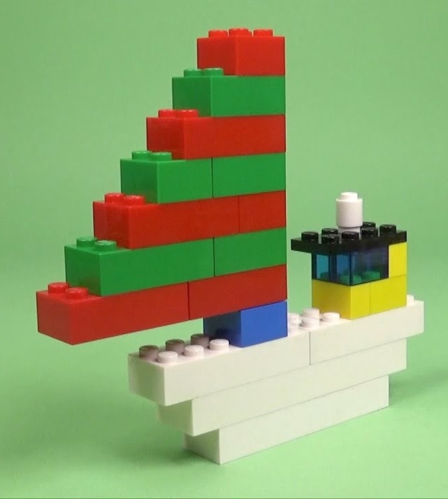
Modeling LEGO units#
We can define a LEGO unit as a small rectangle that contains two cylinders, viewed from above.
It is easy to see that there are \(11\) units vertically.
We can also count that there are \(15\) units horizontally.
Now we need to choose colors for the 2D reconstruction of the LEGO figure. We can use a selection of colors from CSS Colors: Matplotlib CSS Colors
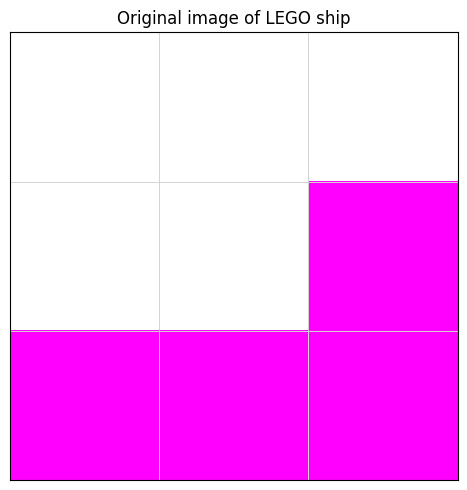
When each LEGO unit and the background are assigned a number corresponding to their color, a \(15\times11\) matrix \(A\) is created, which represents the LEGO figure in 2D.
We assume you will need one color for the background and about seven different colors for the LEGO figure.
Proceed as follows:
In the following cell, in the list
base_colorsreplacewhitewith the colors you have chosen. This assigns the colors a number from \(1\) to \(8\), corresponding to their position in the list. The first color you choose corresponds to the number \(1\), that is, the background color.Then in matrix \(A\) replace each
xwith the number you have chosen for the LEGO unit, so the unit gets the color you want.When you are done, run the cell and the following cells to see your LEGO figure in 2D.
base_colors = ['white','white','white','white','white','white','white','white']

A = np.array([
 [1,1,1,1,1,1,x,x,1,1,1,1,1,1,1],
 [1,1,1,1,1,x,x,x,1,1,1,1,1,1,1],
 [1,1,1,1,x,x,x,x,1,1,1,1,1,1,1],
 [1,1,1,x,x,x,x,x,1,1,1,1,1,1,1],
 [1,1,x,x,x,x,x,x,1,1,1,1,x,1,1],
 [1,x,x,x,x,x,x,x,1,1,x,x,x,x,1],
 [x,x,x,x,x,x,x,x,1,1,1,x,x,x,1],
 [1,1,1,1,1,1,x,x,1,1,1,x,x,x,1],
 [1,1,1,x,x,x,x,x,x,x,x,x,x,x,x],
 [1,1,1,1,x,x,x,x,x,x,x,x,x,x,1],
 [1,1,1,1,1,x,x,x,x,x,x,x,x,1,1]
], dtype=int)
---------------------------------------------------------------------------
NameError                                 Traceback (most recent call last)
Cell In[38], line 4
      1 base_colors = ['white','white','white','white','white','white','white','white']
      3 A = np.array([
----> 4  [1,1,1,1,1,1,x,x,1,1,1,1,1,1,1],
      5  [1,1,1,1,1,x,x,x,1,1,1,1,1,1,1],
      6  [1,1,1,1,x,x,x,x,1,1,1,1,1,1,1],
      7  [1,1,1,x,x,x,x,x,1,1,1,1,1,1,1],
      8  [1,1,x,x,x,x,x,x,1,1,1,1,x,1,1],
      9  [1,x,x,x,x,x,x,x,1,1,x,x,x,x,1],
     10  [x,x,x,x,x,x,x,x,1,1,1,x,x,x,1],
     11  [1,1,1,1,1,1,x,x,1,1,1,x,x,x,1],
     12  [1,1,1,x,x,x,x,x,x,x,x,x,x,x,x],
     13  [1,1,1,1,x,x,x,x,x,x,x,x,x,x,1],
     14  [1,1,1,1,1,x,x,x,x,x,x,x,x,1,1]
     15 ], dtype=int)

NameError: name 'x' is not defined
Hint
Suggestion for coloring:
# Tie colors to numbers + error colors at each end
base_colors = ['palegreen','white','red','forestgreen','blue','yellow','black','cyan']

# Each LEGO unit is assigned a number
A = np.array([
 [1,1,1,1,1,1,3,3,1,1,1,1,1,1,1],
 [1,1,1,1,1,4,4,4,1,1,1,1,1,1,1],
 [1,1,1,1,3,3,3,3,1,1,1,1,1,1,1],
 [1,1,1,4,4,4,4,4,1,1,1,1,1,1,1],
 [1,1,3,3,3,3,3,3,1,1,1,1,2,1,1],
 [1,4,4,4,4,4,4,4,1,1,7,7,7,7,1],
 [3,3,3,3,3,3,3,3,1,1,1,8,8,6,1],
 [1,1,1,1,1,1,5,5,1,1,1,6,6,6,1],
 [1,1,1,2,2,2,2,2,2,2,2,2,2,2,2],
 [1,1,1,1,2,2,2,2,2,2,2,2,2,2,1],
 [1,1,1,1,1,2,2,2,2,2,2,2,2,1,1]
], dtype=int)
# RUN THIS CELL TO SEE YOUR LEGO FIGURE

extended_colors = ['magenta'] + base_colors + ['magenta']
cmap = ListedColormap(extended_colors)

# Define bounds so values <0.5 and >8.5 are shown as magenta
bounds = np.arange(-0.5, len(extended_colors) - 0.5 + 1, 1)
norm = BoundaryNorm(bounds, cmap.N)

# 2) Figure and axes
fig, ax = plt.subplots(figsize=(6,5))

# 3) Draw the image - first the image, then grid (so the grid is on top)
im = ax.imshow(A, cmap=cmap, norm=norm,
               extent=[-0.5, A.shape[1]-0.5, -0.5, A.shape[0]-0.5])

# 4) Create grid with meshgrid + plot
#    x goes from -0.5 to 14.5 (15 columns), y from -0.5 to 10.5 (11 rows)
x = np.arange(-0.5, A.shape[1] + 0.5, 1)
y = np.arange(-0.5, A.shape[0] + 0.5, 1)
X, Y = np.meshgrid(x, y)

ax.plot(X, Y,       color='lightgrey', linewidth=0.7)  # vertical
ax.plot(X.T, Y.T,   color='lightgrey', linewidth=0.7)  # horizontal

# 5) Remove ticks, set uniform aspect, and add a black frame
ax.set_xticks([]); ax.set_yticks([])
ax.set_aspect('equal')

# 6) Title and show
ax.set_title("Original image of LEGO ship")
plt.tight_layout()
plt.show()
Rank-\(k\) matrix approximation#
To compress our LEGO image, we can use SVD on the matrix \(A\):
U, s, Vt = np.linalg.svd(A.astype(float))
By plotting the singular values we get a clear picture of how much each individual term in the sum in \((*)\) contributes to the total matrix.
# Plot singular values
plt.figure(figsize=(8,5))
plt.scatter(np.arange(1, len(s)+1), s, color='blue')
plt.title("Singular values size for A")
plt.xlabel("Index")
plt.ylabel("Singular value size")
plt.grid(True, linestyle='--', alpha=0.5)
plt.show()
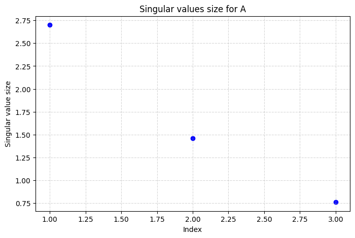
The largest singular values represent the most important patterns in the LEGO image, while the small ones contribute minor details. The plot helps us decide how many singular values we can keep without losing too much information, which is central when we create a \(k\)-rank approximation of the image.
We want to visualize the original LEGO image and rank-\(k\) SVD approximation side by side to see the effect of the approximation.
Complete the function
plot_svd(k)by inserting the functionsvd_approximation()from earlier.
def plot_svd(k):
    # Calculate k-rank approximation of A (called A_recon)
    A_recon = 'INSERT CODE HERE'

    fig, axes = plt.subplots(1, 2, figsize=(12, 5), dpi=100)

    # Create coordinate arrays for pcolormesh - defines the edge of each pixel
    x_edges = np.arange(-0.5, A.shape[1] + 0.5, 1)
    y_edges = np.arange(-0.5, A.shape[0] + 0.5, 1)

    # Create meshgrid for edges
    X, Y = np.meshgrid(x_edges, y_edges)

    # Approximation
    ax = axes[0]
    # Use pcolormesh which naturally aligns with the grid
    mesh = ax.pcolormesh(X, Y, A_recon, cmap=cmap, norm=norm, shading='flat')

    # Add gridlines precisely on edges
    ax.vlines(x_edges, y_edges[0], y_edges[-1], colors='lightgrey', linewidth=0.7)
    ax.hlines(y_edges, x_edges[0], x_edges[-1], colors='lightgrey', linewidth=0.7)

    ax.set_xlim(x_edges[0], x_edges[-1])
    ax.set_ylim(y_edges[0], y_edges[-1])
    ax.invert_yaxis()  # Corrects upside-down image
    ax.set_aspect('equal')
    ax.set_xticks([])
    ax.set_yticks([])
    ax.set_title(f"Approximation with k={k} singular values")

    # Original
    ax = axes[1]
    mesh = ax.pcolormesh(X, Y, A, cmap=cmap, norm=norm, shading='flat')

    ax.vlines(x_edges, y_edges[0], y_edges[-1], colors='lightgrey', linewidth=0.7)
    ax.hlines(y_edges, x_edges[0], x_edges[-1], colors='lightgrey', linewidth=0.7)

    ax.set_xlim(x_edges[0], x_edges[-1])
    ax.set_ylim(y_edges[0], y_edges[-1])
    ax.invert_yaxis()  # Corrects upside-down image
    ax.set_aspect('equal')
    ax.set_xticks([])
    ax.set_yticks([])
    ax.set_title("Original image")

    plt.tight_layout()
    plt.show()
Try different values of \(k\) with the function
plot_svd(k)and see how the image is reconstructed. What effect does it have on the image quality?
# INSERT CODE HERE
Try reconstructing the matrix by including all singular values. Why does it look exactly like the original LEGO image?
Below we investigate how the retained information grows with \(k\) by using the function plot_retained_information() from earlier:
plot_retained_information(A)
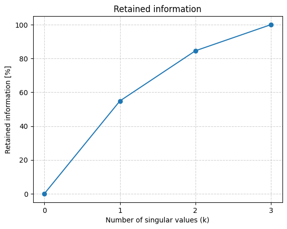
How many singular values should be included to achieve cumulative explanation of over \(90\%\)?
How large does the storage ratio \(L(k,m,n)\) become for the chosen \(k\)?
How is the retained information related to the quality of the image when you change the number of included singular values?
Your Image#
Pixel Values in Images#
An image consists of numbers - each pixel value tells how light or dark that pixel is. In grayscale images, one typically uses integers in the range \(0–255\):
\(0\) = black.
\(255\) = white.
Values in between = gray tones.
For calculations, one often normalizes to the interval \([0, 1]\) by dividing by \(255\). For color images, three such values are stored per pixel (R, G, B), corresponding to one red, one green, and one blue component.
Importing an Image and Data Processing#
For this task, you need to be able to use your own photo.
In this task we work with grayscale images, so your image is converted to grayscale.
def load_image_matrix(path, max_dim=1000, to_gray=True):
    """
    Load an image as a 2D (grayscale) or 3D (RGB) NumPy array in [0,1],
    downscaled so the largest dimension is at most max_dim, with aspect ratio preserved.
    """
    im = Image.open(path)  # Open image file (JPG/PNG etc.)
    if to_gray:
        im = im.convert("L")   # Convert to grayscale
    else:
        im = im.convert("RGB") # Ensure 3 color channels (drops any alpha channel)

    w, h = im.size
    scale = min(1.0, max_dim / max(w, h))  # Calculate scaling factor
    if scale < 1.0:
        # Scale down the image if it is larger than max_dim
        new_size = (max(1, int(round(w * scale))), max(1, int(round(h * scale))))
        im = im.resize(new_size, Image.LANCZOS)

    # Convert to NumPy array with values between 0 and 1
    arr = np.asarray(im, dtype=np.float64)
    arr = arr / 255.0
    return arr

# Load the image
A = load_image_matrix("INSERT FILENAME HERE", max_dim=512, to_gray=True)  # INSERT CODE HERE

plt.imshow(A)
plt.axis("off")  # Hide axes
plt.show()
---------------------------------------------------------------------------
FileNotFoundError                         Traceback (most recent call last)
Cell In[45], line 25
     22     return arr
     24 # Load the image
---> 25 A = load_image_matrix("INSERT FILENAME HERE", max_dim=512, to_gray=True)  # INSERT CODE HERE
     27 plt.imshow(A)
     28 plt.axis("off")  # Hide axes

Cell In[45], line 6, in load_image_matrix(path, max_dim, to_gray)
      1 def load_image_matrix(path, max_dim=1000, to_gray=True):
      2     """
      3     Load an image as a 2D (grayscale) or 3D (RGB) NumPy array in [0,1],
      4     downscaled so the largest dimension is at most max_dim, with aspect ratio preserved.
      5     """
----> 6     im = Image.open(path)  # Open image file (JPG/PNG etc.)
      7     if to_gray:
      8         im = im.convert("L")   # Convert to grayscale

File /builds/ctm/ctmweb/venv/lib/python3.11/site-packages/PIL/Image.py:3512, in open(fp, mode, formats)
   3510 if is_path(fp):
   3511     filename = os.fspath(fp)
-> 3512     fp = builtins.open(filename, "rb")
   3513     exclusive_fp = True
   3514 else:

FileNotFoundError: [Errno 2] No such file or directory: 'INSERT FILENAME HERE'
The cell below prints a data summary for the image.
# Data summary for the image
print('Object type:\n',type(A))
print('Dimensions:\n',A.shape)
print('Data type of elements:\n',A.dtype)
print('Data range:\n',[np.min(A), np.max(A)])
Object type:
 <class 'numpy.ndarray'>
Dimensions:
 (3, 3)
Data type of elements:
 int64
Data range:
 [-1, 2]
Run the cell above and consider the dimensions. Do they make sense?
SVD on images#
With the correct matrix representation of the image, we can now examine the rank of the matrix.
print("Rank of matrix:\n", np.linalg.matrix_rank(A))
Rank of matrix:
 3
How many non-zero singular values can we expect?
We perform SVD on the image:
U, s, Vt = np.linalg.svd(A)
Sigma = np.diag(s) # diagonal matrix with s as diagonal entries
Display the size of the singular values in a plot.
# INSERT CODE HERE
What does it mean that the first singular value is often much larger than the next ones?
Like in the LEGO ship exercise, we will now examine the singular values based on the retained information. See the plot below.
plot_retained_information(A)
Read from the plot what the number of singular values should be to achieve \(90 \%\), \(95 \%\), and \(99 \%\) of the retained information respectively.
Construction of approximated images#
We want to construct approximations of the original black-and-white image by using only the first \(k\) singular values.
We will examine the quality of the approximations when different numbers of singular values are used.
Use the function
svd_approximation()to complete the functionplot_approximation()below.
The function plots the rank-\(k\) approximation and the original image side by side.
def plot_approximation(A,k):
    # Rank-k reconstruction via outer products
    A_recon = 'INSERT CODE HERE'

    # Figure with two plots
    fig, axes = plt.subplots(1, 2, figsize=(10,5))

    # Approximation
    ax = axes[0]
    ax.imshow(A_recon, cmap='gray', interpolation='nearest')
    ax.set_title(f'Rank-{k} approximation')
    ax.set_xticks([]); ax.set_yticks([])

    # Original
    ax = axes[1]
    ax.imshow(A, cmap='gray', interpolation='nearest')
    ax.set_title('Original')
    ax.set_xticks([]); ax.set_yticks([])

    plt.tight_layout()
    plt.show()
Experiment with the number of singular values and use the function plot_approximation(A,k) to answer the following:
How many singular values should be used before the subject can be recognized?
How many should be used before you can see details?
How many should be used before the approximation is as good as the original image to the naked eye.
What does that correspond to in retained information \(RI\) and storage ratio \(SR(k,m,n)\)?
Can you recognize elements in the image in the approximation if only the first singular value is used? E.g., sky/land, background/foreground, etc.
Challenging: Color approximation with SVD#
In the previous exercises, we only worked with grayscale or 2D LEGO matrices. Real images typically consist of three color channels: Red (R), Green (G), and Blue (B). Each channel can be treated as a matrix where we can perform SVD and create a rank-\(k\) approximation.
By doing this for all three channels individually and putting them back together, we can create a compressed version of the color image. This clearly shows how SVD can be used for image compression in color. Our procedures svd_approximation(), retained_information(), and plot_retained_information() must therefore be extended to handle 3 channels.
The assignment is therefore:
Divide your image into R, G, and B channels.
Perform SVD on each channel.
Create a rank-\(k\) approximation for each channel.
Reassemble the channels to recreate the image.
Visualize the result.
def svd_rgb_approximation(img, k, verbose=False):
    """
    Returns a rank-$k$ SVD approximation of an RGB image.

    Parameters:
    - img: an RGB image as a numpy array (height x width x 3)
    - k: number of singular values to include per channel

    Returns:
    - img_recon: the approximated image
    """
    img = np.asarray(img)

    # Convert the image to float with the same size
    imgf = img.astype(float)

    # Create a copy of the image that we can fill with the approximation - use np.zeros_like
    img_recon = 'INSERT CODE HERE'

    # Go through the three color channels (R, G, B)
    for i in range(3):
        # Calculate k-rank approximation for this channel - use svd_approximation(channel, k)
        channel = imgf[:, :, i]
        Xk = 'INSERT CODE HERE'
        img_recon[:, :, i] = Xk

    # Ensure that pixel values are within 0–1 - use np.clip
    img_recon = 'INSERT CODE HERE'

    return img_recon


A = load_image_matrix("INSERT FILENAME HERE", max_dim=512, to_gray=False)
img_recon = svd_rgb_approximation(A, k=100, verbose=True)

# Visualize the result
plt.figure(figsize=(6,5))
plt.imshow(img_recon)
plt.title("RGB rank-k approximation")
plt.axis('off')
plt.show()
---------------------------------------------------------------------------
FileNotFoundError                         Traceback (most recent call last)
Cell In[52], line 33
     28     img_recon = 'INSERT CODE HERE'
     30     return img_recon
---> 33 A = load_image_matrix("INSERT FILENAME HERE", max_dim=512, to_gray=False)
     34 img_recon = svd_rgb_approximation(A, k=100, verbose=True)
     36 # Visualize the result

Cell In[45], line 6, in load_image_matrix(path, max_dim, to_gray)
      1 def load_image_matrix(path, max_dim=1000, to_gray=True):
      2     """
      3     Load an image as a 2D (grayscale) or 3D (RGB) NumPy array in [0,1],
      4     downscaled so the largest dimension is at most max_dim, with aspect ratio preserved.
      5     """
----> 6     im = Image.open(path)  # Open image file (JPG/PNG etc.)
      7     if to_gray:
      8         im = im.convert("L")   # Convert to grayscale

File /builds/ctm/ctmweb/venv/lib/python3.11/site-packages/PIL/Image.py:3512, in open(fp, mode, formats)
   3510 if is_path(fp):
   3511     filename = os.fspath(fp)
-> 3512     fp = builtins.open(filename, "rb")
   3513     exclusive_fp = True
   3514 else:

FileNotFoundError: [Errno 2] No such file or directory: 'INSERT FILENAME HERE'
We want to investigate how the retained information develops for each of the three color channels in an RGB image. This provides insight into which channels carry the most information, and how much rank-\(k\) approximation can compress the image without significant loss of quality.
Perform SVD for each channel (Red, Green, Blue).
Calculate the associated retained information for each channel.
Plot the results together and assess how many singular values should be used to achieve \(90 \%\) of the retained information in each channel.
# Plot cumulative variance explained for the RGB image with channel-specific color
channels = ['Red', 'Green', 'Blue']
colors = ['red', 'green', 'blue']
plt.figure(figsize=(8,5))

for i, (channel, color) in enumerate(zip(channels, colors)):
    # Perform SVD on each channel
    'INSERT CODE HERE'

    # Calculate the associated cumulative information
    'INSERT CODE HERE'

    # Plot cumulative information
    'INSERT CODE HERE'


plt.xlabel('Number of singular values included')
plt.ylabel('Retained information')
plt.title('Retained information per color channel')
plt.axhline(0.9, color='black', linestyle=':', label='90% line')
plt.legend()
plt.grid(True, linestyle='--', alpha=0.5)
plt.show()