import matplotlib
if not hasattr(matplotlib.RcParams, "_get"):
    matplotlib.RcParams._get = dict.get
Theory#
Networks show up everywhere: transport systems, communication networks, power grids, social connections, and dependencies between tasks.
Mathematically, we model a network as a graph.
A graph is a pair \(G=(V,E)\) where:
\(V\) is a set of nodes (also called vertices),
\(E\) is a set of edges connecting pairs of nodes.
In this project we mainly think of undirected graphs, where an edge \((u,v)\) means “\(u\) is connected to \(v\)” and the order does not matter.
Basic graph language#
Nodes, edges, and neighbors#
Two nodes \(u\) and \(v\) are neighbors if \((u,v)\in E\).
The degree of a node \(v\) (written \(\deg(v)\)) is the number of neighbors of \(v\).
A key counting fact is the handshaking lemma:
So the sum of degrees is always even, and it equals twice the number of edges.
Simple graphs, multi-graphs, and loops#
A simple graph has:
no multiple edges between the same pair of nodes,
no loops \((v,v)\).
networkx.Graph() is a simple undirected graph (it prevents duplicate edges, and loops are allowed but usually avoided unless we really want them).
Directed graphs (optional perspective)#
In a directed graph (a digraph), edges are ordered: \(u\to v\).
Then we distinguish:
out-degree: number of edges leaving \(u\),
in-degree: number of edges entering \(u\).
In networkx, directed graphs use nx.DiGraph().
Ways to represent a graph#
Edge list#
List all edges: $\( E = \{(A,B),(A,D),(B,C),\dots\}. \)$ This is the most compact “human readable” representation.
Adjacency list#
For each node, store its neighbors. For example: $\( N(A)=\{B,D\},\quad N(B)=\{A,C\},\dots \)$ This is efficient for traversal (like BFS).
Adjacency matrix#
If we number nodes \(1,\dots,n\), we can represent the graph as a matrix \(A\in\{0,1\}^{n\times n}\) where
For an undirected graph, \(A\) is symmetric.
Walks, paths, and distance#
Walk and path#
A walk of length \(k\) is a sequence of nodes $\( v_0, v_1, \dots, v_k \)\( such that each consecutive pair is an edge: \)(v_{i-1},v_i)\in E$.
A path is a walk where all nodes are distinct (no repeats).
Distance and shortest path#
The distance between nodes \(u\) and \(v\) (written \(\operatorname{dist}(u,v)\)) is the length of the shortest path from \(u\) to \(v\).
If no path exists, the distance is undefined (or we treat it as \(\infty\)).
This happens exactly when \(u\) and \(v\) lie in different connected components.
Breadth-first search (BFS)#
For unweighted graphs, the standard way to compute shortest-path distances from a start node \(s\) is breadth-first search (BFS).
Intuition:
First discover all nodes at distance \(1\) from \(s\),
then all nodes at distance \(2\),
and so on “layer by layer”.
BFS returns:
a distance to every reachable node,
often also a parent (predecessor) that lets you reconstruct actual shortest paths.
Complexity idea#
If the graph has \(|V|\) nodes and \(|E|\) edges, BFS runs in
which is essentially linear in the size of the graph.
Connectedness and connected components#
A graph is connected if there is a path between every pair of nodes.
If a graph is not connected, it splits into connected components: maximal sets of nodes where every pair is connected by some path.
You can find the connected component containing a node \(s\) by running BFS from \(s\) and collecting all nodes with finite distance.
Graphs in Python with networkx#
Below is a minimal “reference” for the most common operations used in the project.
Setup#
import networkx as nx
import matplotlib.pyplot as plt
Creating a graph, adding nodes and edges#
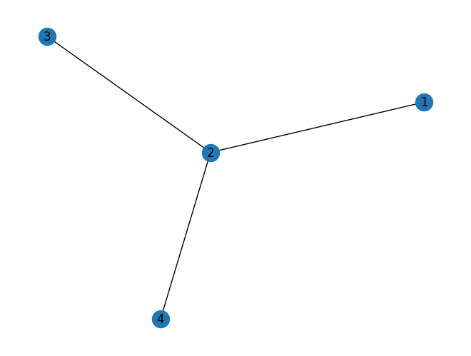
G = nx.Graph()

# Nodes (optional: edges auto-create nodes too)
G.add_nodes_from([1, 2, 3, 4])

# Edges
G.add_edge(1, 2)
G.add_edge(2, 3)
G.add_edge(2, 4)

# Draw
nx.draw(G, with_labels=True)
plt.show()
Inspecting structure: nodes, neighbors, degrees#
print("Nodes:", list(G.nodes()))
print("Edges:", list(G.edges()))
print("Neighbors of 2:", list(G.neighbors(2)))
print("Degree of 2:", G.degree[2])

# Handshaking lemma check: sum of degrees = 2|E|
sum_deg = sum(G.degree[v] for v in G.nodes())
print("Sum of degrees:", sum_deg, " = 2|E| =", 2 * G.number_of_edges())
Nodes: [1, 2, 3, 4]
Edges: [(1, 2), (2, 3), (2, 4)]
Neighbors of 2: [1, 3, 4]
Degree of 2: 3
Sum of degrees: 6  = 2|E| = 6
Shortest paths in networkx#
For unweighted graphs, networkx uses BFS internally.
# Distance (shortest path length)
d = nx.shortest_path_length(G, source=1, target=4)
print("dist(1,4) =", d)

# One shortest path
path = nx.shortest_path(G, source=1, target=4)
print("A shortest path 1->4:", path)
dist(1,4) = 2
A shortest path 1->4: [1, 2, 4]
If you want distances from one node to all reachable nodes:
distances = dict(nx.shortest_path_length(G, source=1))
print("Distances from node 1:", distances)
Distances from node 1: {1: 0, 2: 1, 3: 2, 4: 2}
Connected components in networkx#
# Create a disconnected graph
H = nx.Graph()
H.add_edges_from([(0,1), (1,2), (5,6)])

components = list(nx.connected_components(H))
print("Connected components:", components)
print("Number of components:", nx.number_connected_components(H))

# Is it connected?
print("Is H connected?", nx.is_connected(H))
Connected components: [{0, 1, 2}, {5, 6}]
Number of components: 2
Is H connected? False