Computed Tomography#
About the project#
Duration: 20–50 hours (including typesetting final report in LaTeX)
Prerequisites: Differential equations (1st order), multivariable calculus (line integrals, change of variables), linear algebra (matrices, null space/column space, least squares), basic numerical methods, basic Python programming
Python packages: NumPy, matplotlib, scipy, sympy
Learning objectives: Model X-ray attenuation via Lambert’s law, formulate and analyze the Radon transform, interpret sinograms and backprojection, implement filtered backprojection, discretize line integrals as sparse matrices, and solve inverse problems via least squares and regularization
Important
This project was created by by Bjørn Jensen and Kim Knudsen.
This notebook describes a project on CT scanning. It may be a good idea to start by looking at the introduction at http://ct-srp.compute.dtu.dk/; it is material behind an outline on the same topic (at a lower level).
Good luck!
1 Introduction#
Computed Axial Tomography (CAT), or simply computed tomography, abbreviated CT, is a powerful image-processing technique with both medical and industrial applications. While there are many different computer-based tomography technologies, CT typically (and also here) refers to X-ray tomography.
The most widely known application of CT is in medical imaging, where it is used for brain imaging, cancer detection, lung problems, heart anatomy, and especially complex bone fractures. Of course, this list is not exhaustive. CT is also used in industry in various ways, for example for 3D reconstruction and defect detection in components. Another interesting application is inspection of underwater pipelines. In this application a robot is sent to the seabed to monitor possible cracks or weak places in the pipe. Finally, CT is used for studying materials. In particular, grain structures can be found using high-intensity CT instruments, also known as synchrotrons. In fact, some new large facilities are currently being built in Lund (synchrotron MAX IV and neutron facility ESS) in close collaboration with DTU. The applications are very diverse; so are the instruments and the scale. The mathematics is, however, surprisingly similar, and that is what we will focus on here.
Exercise 1.
Briefly discuss the societal importance of CT scans, e.g. in medical imaging. (Use e.g. online sources.)
A CT image visualizes a certain physical property of the imaged object. More precisely, it visualizes X-ray absorption, also known as the attenuation coefficient \(\mu\). This is a function in 3D, \(\mu(x,y,z)\), that can take different values from region to region in the body depending on local tissue, organs, bones, etc. The purpose of CT is to create images of this function non-invasively, i.e. without subjecting the patient to surgery.
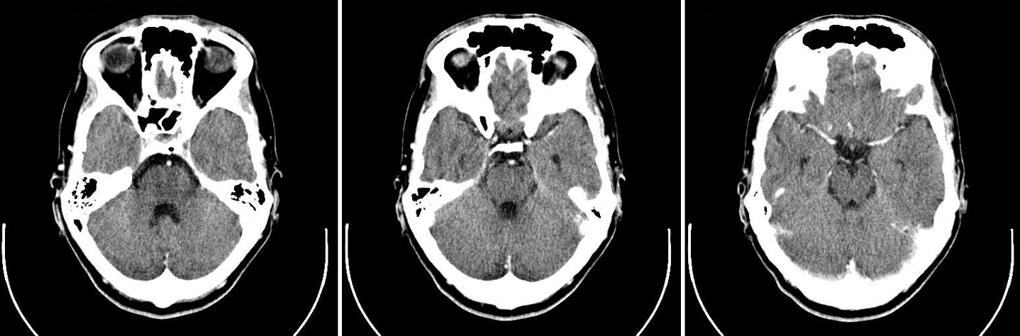
Figure 1: 2D slices of a human head from a CT scan.
Figure 1 contains brain CT images taken at different “horizontal” slices through the patient. In the images in Figure 1 the slices follow planes perpendicular to the foot-to-head direction. Each grayscale image is interpreted as a contour plot of the function \(\mu(x,y,z_0)\) in the plane \(z=z_0\).
Now we know what we are looking at in Figure 1, but we are not able to access these images (slices) directly. Instead, we take X-ray measurements outside the patient, and the goal is to determine the internal attenuation coefficient from external measurements by solving an inverse problem.
The following project description starts with a warm-up on number puzzles. Then it falls into three parts: first we consider the mathematical modeling of X-rays and attenuation, then we focus on the mathematical analysis of the model, and finally we consider numerical computations that open for deeper insight into larger problems.
2 Warm-up: Number puzzles#
To get an idea of the basics, consider the number puzzle in Figure 2. The goal is to determine the cell values so that the row and column sums are equal to (5, 2) and (3, 4), respectively. Four linear equations for four unknown variables call for matrices and linear algebra.
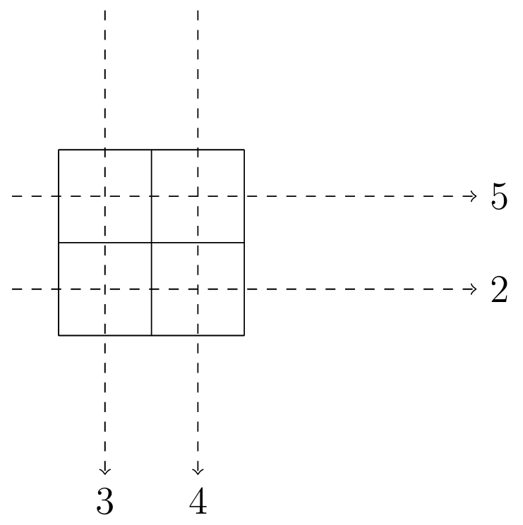
Figure 2: A \(2\times 2\) grid puzzle.
Exercise 2.
Set up the corresponding matrix equation and solve the puzzle in Figure 2. Discuss the form of the solution in terms of the column space and null space of the associated matrix.
Hopefully you can see that the problem has many solutions, but then we can use prior information:
Exercise 3.
Assume that we know that the cell values are positive integers. Find the unique solution to the puzzle in Figure 2.
Similar puzzles can be set up for larger systems, see the \(3\times 3\) problem in Figure 3. Here we have 6 equations for 9 unknowns. But then we can add more sums, for example along the diagonal, see Figure 4.
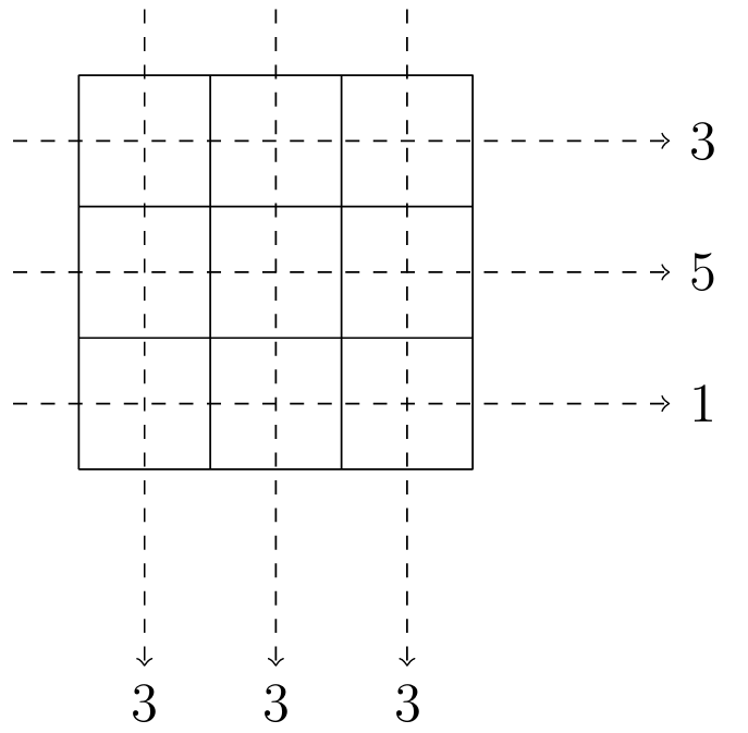
Figure 3: A \(3\times 3\) grid puzzle.
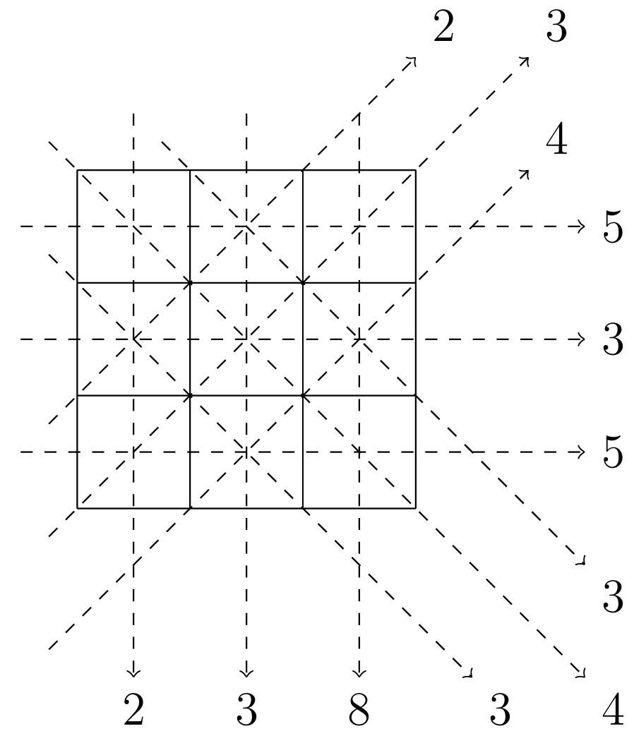
Figure 4: A \(3\times 3\) grid puzzle with diagonal sums.
Exercise 4.
Solve the puzzles in Figure 3 and in Figure 4.
This small puzzle contains much of what we will work with on the following pages. The grid represents a small bounded domain with an unknown function (here the function is piecewise constant in each grid square), and we want to determine this function by knowing the sum of its values along some lines. Imagine that we refine the grid. When we do that, we will naturally need more and different lines to sum over in order to guarantee that we can find a solution, since the number of unknowns will increase.
3 Mathematical modeling#
In the following sections we will look at the physics behind attenuation and derive a mathematical model. This involves differential equations and line integrals of functions. Then we define the Radon transform and study its different properties.
3.1 Lambert’s law#
The intensity of a ray describes the energy in the ray, which depends on the number of photons it carries. Absorption of photons is a matter of probability. Suppose that a photon is absorbed in a slab of material \(M\) with probability \(p\), then the probability of absorption increases if we arrange a sequence of multiple copies of \(M\). Given \(n\) slabs of \(M\), standard probability calculus gives an absorption probability of \(1-(1-p)^n\). However, a ray contains enough photons that probabilities can be neglected in favor of the mean value.
Consider the situation shown in Figure 5. An X-ray beam moves along the \(x\)-axis with initial intensity \(I_0\). To model the loss of intensity and in particular the intensity \(I(x)\) at a point \(x\), we consider a thin slab of material with thickness \(\Delta x=x_2-x_1\). The intensity change over the slab is then \(\Delta I = I(x_2)-I(x_1)\). This change is proportional to the incident intensity \(I=I(x_1)\) and the thickness of the slab, i.e. \(\Delta I \propto I\Delta x\). The proportionality constant is \(-\mu\), where \(\mu\ge 0\), i.e.
This is Lambert’s law, named after Johann Heinrich Lambert in 1760, although it was actually discovered earlier by Pierre Bouguer, who published it in 1729, from where Lambert cited it.
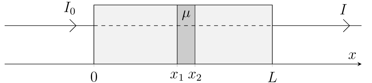
Figure 5: A ray entering an object. In the middle of the object a slab is assumed to have constant attenuation coefficient \(\mu\).
Exercise 5.
Discuss the meaning of the sign in the coefficient \(-\mu\).
Exercise 6.
Derive the differential equation\[\begin{equation*} I'(x) = -\mu(x)I(x),\qquad I(0)=I_0. \qquad \text{(2)} \end{equation*}\]
The coefficient \(\mu\) is the non-negative absorption coefficient (attenuation coefficient), and in the case of soluble substances one has \(\mu = \ln(10)\,\varepsilon\,C\), where \(C\) is the concentration of the substance and \(\varepsilon\) is called the molar extinction coefficient. This relationship for soluble substances is Beer’s law after August Beer in 1852. The two laws are sometimes mentioned together as Lambert–Beer’s law.
As Beer’s law shows, \(\mu\) can depend on many different parameters. A well-known dependence, which we ignore in this project, is the ray’s frequency. X-rays are a form of electromagnetic radiation, like visible light, but vary in wavelength from 0.01 to 10 nanometers. Different wavelengths correspond to different frequencies \(\omega\), and the material can attenuate differently for these, \(\mu=\mu(\omega)\). We will assume that \(\omega\) is constant, which is only true in large synchrotron facilities, but this is one of many simplifications of the model we will use.
Exercise 7.
Let us solve the differential equation (2):
Determine \(I(x)\) as a function of \(I_0\) and \(\mu(x)\). You may assume \(\mu=0\) for \(x<0\) and \(x>L\).
Let \(I_1=I(L)\) denote the exit intensity. Show that
\[\begin{equation*} \ln\left(\frac{I_1}{I_0}\right) = -\int_0^L \mu(x)\,dx. \end{equation*}\]
It should be clear that everything is about integrals along ray paths, and therefore we need to go deeper into line integrals.
3.2 Line integrals#
The basis of CT mathematics is the Radon transform, named after the Austrian mathematician Johann Radon, who developed the mathematical theory in 1917. The Radon transform takes a function \(f:\mathbb{R}^2\to\mathbb{R}\) and maps it to a collection of line integrals of the same function. Therefore our first task is to describe a line \(\ell\) in \(\mathbb{R}^2\).
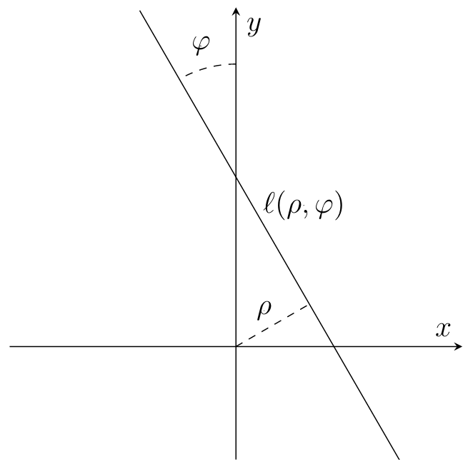
Figure 6: The line \(\ell(\rho,\varphi)\).
Exercise 8.
Let \(\ell(\rho,\varphi)\) denote the line in \(\mathbb{R}^2\) with angle \(\varphi\) counterclockwise from the \(y\)-axis and signed distance \(\rho\) from the origin, as shown in Figure 6. Note that this means \(\rho\) can be negative.(a) Draw a coordinate system with a representative line and mark the parameters \(\rho\) and \(\varphi\) in the drawing. The angle \(\varphi\) appears in several places—can you identify them?
(b) Write an equation for the line \(\ell(\rho,\varphi)\).
(c) Give a parameterization \(r_\ell(t)\) of \(\ell(\rho,\varphi)\).
With this in place we choose a function \(f:\mathbb{R}^2\to\mathbb{R}\) and denote by \(p_\varphi(\rho)\) the line integral of \(f\) along \(\ell(\rho,\varphi)\), i.e.
Exercise 9.
Use your parameterization from Exercise 8 to write out the integral expression for \(p_\varphi(\rho)\).
Before we proceed, let us define a function that is convenient to work with.
The rectangle function is defined as
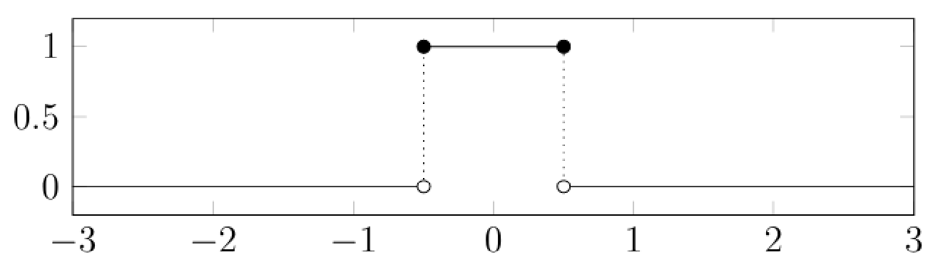
Figure 7: Plot of \(\mathrm{rect}(t)\).
Exercise 10.
Verify that \(f(x,y)=\mathrm{rect}\left(\dfrac{\sqrt{x^2+y^2}}{2}\right)\) defines the unit disk. Determine the line integrals \(p_\varphi(\rho)\).
(Tip: Use the symmetry of the unit disk.)
Exercise 11.
Let \(f(x,y)=\mathrm{rect}(x)\,\mathrm{rect}(y)\) and compute the line integrals \(p_{\pi/3}(\rho)\).
Although it was not explicitly mentioned, we have in fact computed the Radon transform of the function \(f\) by solving Exercise 10 above. Let us define it more precisely.
4 Mathematical analysis#
First we define the support of a function.
Definition 1. The support of a function \(f(x,y)\) is the smallest closed set \(K=\mathrm{supp}(f)\subset\mathbb{R}^n\) such that \(f(x,y)=0\) for \((x,y)\in\mathbb{R}^n\setminus K\). A function \(f\) is said to have compact support if \(\mathrm{supp}(f)\) is bounded.
The function
is an example of a function in \(C_C(\mathbb{R}^2)\).
Exercise 12.
Check that \(f_1\in C_C(\mathbb{R}^2)\) and state \(\mathrm{supp}(f_1)\). Give another example of a function in \(C_C(\mathbb{R}^2)\).
Exercise 13.
Show that \(C_C(\mathbb{R}^2)\) is a vector space. What is the dimension of \(C_C(\mathbb{R}^2)\)?
(Tip: How many linearly independent elements can you find?)
It is often useful to go from the function \(f(x)\) and the line integrals \(p_\varphi(\rho)\) to the mapping (operator) that connects any \(f\) to its \(p\):
Definition 3 (Radon transform). The Radon transform is the operator \(R:C_C(\mathbb{R}^2)\to C_C(\mathbb{R}\times\mathbb{T})\), \(Rf(\rho,\varphi)=p_\varphi(\rho)\), defined by
Note that \(p\) is defined on the domain \(\mathbb{R}\times\mathbb{T}\). \(\mathbb{T}\) is the circle, which conveniently defines the direction/angle \(\varphi\). You can think of \(\mathbb{T}\) as the interval \([0,2\pi)\), but looped, so if you move out of the interval at one end, you immediately come back at the other end; corresponding to a circle.
Exercise 14.
Show that if \(f\) has compact support, then the Radon transform \(r=Rf\) also has compact support in \(\rho\), i.e. show that there exists \(\rho_0>0\) such that \(r(\rho,\varphi)=0\) for all \(\rho>\rho_0\).
Exercise 15.
Relate the above definition of the Radon transform to Lambert’s law derived in Exercise 7.
4.1 Properties of the Radon transform#
A remarkable property of the Radon transform is that it is invertible. That is, \(r(\rho,\varphi)\) actually contains all the information required to reconstruct \(f(x,y)\). So if we know \(r\) from measurements, we can also determine \(f\). We return to this later. Now we look at some other properties.
Exercise 16 (Linearity).
Show that the Radon transform is a linear operator.
Exercise 17 (Translation property).
Show that if \(r=Rf\) and \(\tilde f(x,y)=f(x-x_0,y-y_0)\) is a shifted \(f\), then \(R\tilde f=\tilde r\), where \(\tilde r(\rho,\varphi)=r(\rho-x_0\cos\varphi-y_0\sin\varphi,\varphi)\).
(Tip: Use your result from Exercise 9.)
Exercise 18 (Rotation property).
Show that if \(r=Rf\) and \(f_\theta\) is \(f\) rotated about the origin by angle \(\theta\), then \(Rf_\theta=r_\theta\), where \(r_\theta=r(\rho,\varphi-\theta)\).
(Tip: (i) Write \(f_\theta\) as \(f\circ M_\theta\) where \(M_\theta\) is a rotation matrix. (ii) Use your result from Exercise 9. (iii) Use the trigonometric angle-sum identities.)
Exercise 19 (Scaling property).
Let \(\alpha>0\). Show that if \(r=Rf\) and \(f_\alpha(x,y)=f(\alpha x,\alpha y)\), then \(Rf_\alpha=r_\alpha\), where \(r_\alpha(\rho,\varphi)=\dfrac{1}{\alpha}r(\alpha\rho,\varphi)\).
4.2 Sinogram#
The measurements in a CT scan, \(r(\rho,\varphi)\), can be studied in different ways. Typically we make a contour plot, the so-called sinogram. It is a 2D plot in the \((\rho,\varphi)\) coordinate system. See Figure 8 for a computed example of an image and corresponding sinogram. Note the oscillating sine/cosine patterns in the sinogram.
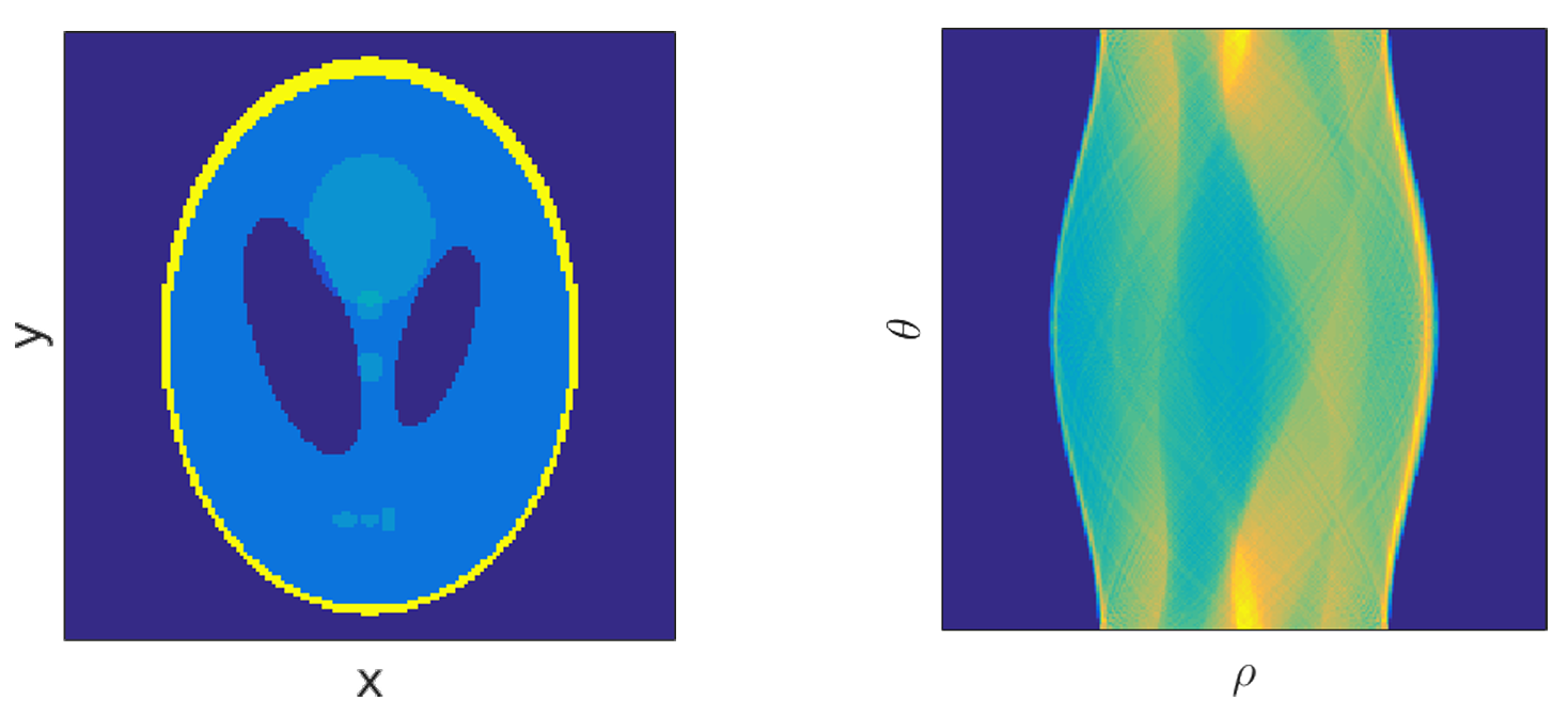
Figure 8: Shepp–Logan phantom and corresponding sinogram.
We are particularly interested in understanding the contribution to \(r(\rho,\varphi)\) from function values at a single point \((x_0,y_0)\). We call this the point’s signature. See also Figure 9.
Exercise 20.
Identify how the points and curves correspond.
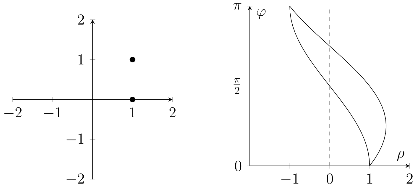
Figure 9: Left: two points. Right: the corresponding Radon transforms (a line integral through one of the two points evaluates to 1).
The purpose of the following exercise is to understand the terminology “sinogram”.
Exercise 21 (Sinogram).
Consider a point \((x_0,y_0)\).
Find an equation in the \((\rho,\varphi)\)-plane for the curve that describes all lines that pass through the point \((x_0,y_0)\).
Interpret the curve as a sine/cosine function.
Define a “function” \(f\) that is infinite at the point \((x_0,y_0)\) and zero everywhere else; but with the remarkable property that the integral of \(f\) along any line that passes through \((x_0,y_0)\) is identically 1. (This is called the Dirac delta function.)
How do you expect the sinogram \(r(\rho,\varphi)\) to look?
Exercise 22.
Note that in Figure 9 we only plot \(\varphi\) in the interval \((0,\pi)\). Consider the geometry and how \(r\) looks in the interval \((\pi,2\pi)\), and why the illustrated interval is sufficient.
Exercise 23.
In Figure 9 the points are located at \((1,0)\) and \((1,1)\). Determine parameterizations for the shown curves.
4.3 Backprojection#
Now that we can compute Radon transforms, we of course also want to be able to return to the original function. That is, we want an inverse Radon transform. We have already touched on the existence of the inverse transform, but it is not obvious how to do it.
From the geometry of a function and its profile curves, an intuition may be to “smear” the profile curves back across the domain along their corresponding ray directions. This is commonly called backprojection. That is, at each point \((x,y)\) the backprojection is the average of all line integrals that pass through the point. Although it is not a true inverse image, it still produces something that resembles the original image, even though it is blurred. In fact, we can determine precisely what goes wrong.
Definition 4. Let \(r=Rf\) be the Radon transform of \(f\) and \(f_b\) the backprojection, then
To see what backprojection actually does, we first need the following result.
Exercise 24.
Show that if \(g(x,y)=f(x-x_0,y-y_0)\) then \(g_b(x,y)=f_b(x-x_0,y-y_0)\).
This result tells us that backprojection works the same way everywhere, which means it is enough to investigate its effect at a single point, e.g. at \((0,0)\).
Exercise 25.
Show that\[\begin{equation*} f_b(0,0)=\iint_{-\infty}^{\infty} \frac{1}{\sqrt{x^2+y^2}}\,f(-x,-y)\,dx\,dy, \end{equation*}\]i.e. \(f_b\) is the 2D convolution of \(h(x,y)=(x^2+y^2)^{-1/2}\) with \(f\), \(f_b(x,y)=(h\ast f)(x,y)\).
(Tip: Use the definition of \(f_b\) and the Radon transform and perform a coordinate change.)
So we can see that backprojection produces the correct \(f\), but with a blurring operator applied. That is why it looks right at first glance, but loses the sharpness that the original \(f\) could have had.
4.4 Filtered backprojection#
By filtering the backprojection we can remove the blurring effect. This is best described using the Fourier transform; this is a topic taught in depth in later mathematics courses, and we will only touch the surface here.
Definition 5 (1D Fourier transform). Let \(g:\mathbb{R}\to\mathbb{R}\). The Fourier transform of \(g\), denoted \(\hat g\), is
The inverse Fourier transform is
As the notation indicates, one can show that
The Fourier transform is widely used in mathematics and signal processing; it captures the frequency content of the function \(g\).
Exercise 26.
Write the definition of the Fourier transform using \(\sin\) and \(\cos\) instead of the complex exponential function.
A filter in signal processing is often defined by a filter function \(\psi(\xi)\) through multiplication in the Fourier domain.
Definition 6 (Filter). The filtering of the function \(g\) by the filter \(\psi\) is defined by
The special filter function \(\psi(\xi)=|\xi|\) is called the ramp filter. It is important for the following result, called the filtered backprojection formula. Assume the function \(f\) has Radon transform \(Rf=r(\rho,\varphi)\). Then we find the inversion by first filtering and then applying backprojection:
Exercise 27.
Write a complete formula (with integrals) that gives \(f(x,y)\) from its Radon transform \(r(\rho,\varphi)\).
Exercise 28.
Implement the formula in Python and experiment with different functions \(f(x)\); also experiment with other filter functions \(\psi(\xi)\), different from the ramp filter.
5 Numerical implementation and computations#
In the previous section we discussed the Radon transform and integral representations. Integration is a linear operation, which in a discretized model means it can be represented by matrix multiplication. But how do we do this?
Let us reconsider the number puzzle in Figure 4. Assume the \(3\times 3\) grid represents a function that is constant in each cell (and zero outside). Assume the cells have dimension \(1\times 1\) (you choose the units). Write down the line integral along the diagonal (introduce unknown variables \(x_1,x_5,x_9\)).
Exercise 29.
Modify the diagonal sums in Figure 4 to account for the length of the diagonal inside each cell (with length \(\sqrt{2}\)). Solve the resulting system of linear equations.
There are multiple ways to approach discretizing the theory. A common feature is that we must move to a finite-dimensional vector space.
5.1 The grid#
We assume our function can be approximated by something piecewise constant on a square grid. This is completely analogous to the puzzle in Figure 4 that we solved earlier. We will, however, allow more freedom with the lines through the grid and additional weighting of the contribution from each grid cell by the distance the line travels through that particular cell.
Exercise 30.
Let \(a>0\) and define the box \(B=\{(x,y)\in\mathbb{R}^2\mid x,y\in(-a,a]\}\).(a) Illustrate the set \(B\).
(b) Let \(N\in\mathbb{N}\) and create a uniform grid on \(B\) that divides it into \(N^2\) equal cells \(C_{ij}\); determine the set \(C_{ij}\). (Note: \(C_{ij}\) should be constructed with half-open intervals \((\cdot,\cdot]\), like \(B\).)
We work with functions that are constant on each cell \(C_{ij}\). Let \(\chi_{C_{ij}}\) be the indicator function of \(C_{ij}\), i.e.
Then \(V=\mathrm{span}_{ij}\{\chi_{C_{ij}}\}\) is our finite-dimensional vector space, and a function \(f\in V\) can be viewed as a finite-dimensional vector
or as a function where the vector components are coefficients:
5.2 Matrix representation of the Radon transform#
Now that we have partitioned our function and represented it as a vector, the Radon transform, which we remember as a linear operator, can be represented by a matrix \(A\). In this section we determine how to compute this matrix.
Looking back at the puzzle in Figure 4, the matrix used to solve that problem was
Notice how each summation line through the grid corresponds to a row of \(A\) and each column corresponds to a cell in the grid. Only the crossed cells give non-zero entries. Clearly such a matrix will be very sparse (mostly zeros). We seek something similar here, although the lines have more freedom in their placement, and the matrix elements will be proportional to the lengths of the line segments that intersect the cells.
To find \(A\) we first find the interactions between our “rays” \(\ell(\rho,\theta)\) and the individual cells in the grid.
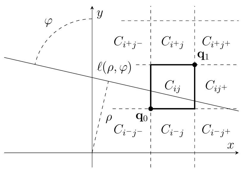
Figure 10: Illustration of a line \(\ell(\rho,\varphi)\) passing through a cell \(C_{ij}\). Here \(\pm\) is shorthand for \(i\pm 1\); similarly for \(j\).
Exercise 31.
Given the line \(\ell(\rho,\varphi)\) and the cell \(C_{ij}\), let \(q_0=(x_0,y_0)\) and \(q_1=(x_1,y_1)\) be the lower-left and upper-right corners of \(C_{ij}\), respectively, see Figure 10. Determine a way to check whether the line \(\ell(\rho,\varphi)\) passes through \(C_{ij}\).
Exercise 32.
Assume that the line \(\ell(\rho,\varphi)\) passes through the cell \(C_{ij}\). Determine the length of the line segment that passes through \(C_{ij}\).
Exercise 33.
Based on your solutions above, write a Python function
intersect_cell(i,j,a,N,rho,theta)
that checks whether the line \(\ell(\rho,\theta)\) intersects the cell \(C_{ij}\).
Exercise 34.
Based on your solutions above, write a Python function
get_length(i,j,a,N,rho,theta)
that, if the line \(\ell(\rho,\theta)\) crosses the cell \(C_{ij}\), computes the length of the line segment in the cell.
Assume we have labeled all ray lines \(\ell_k\equiv\ell(\rho_k,\theta_k)\), \(1\le k\le M\). Let \(s_{ij,k}\) be the length of the segment of line \(k\) that passes through cell \(C_{ij}\). Then we can construct a matrix in which each row corresponds to a single “ray”, i.e.
and we can interpret the equation \(Ax=b\) as the Radon transform of the function \(f\in V\) corresponding to \(x\) according to (6)–(7).
Exercise 35.
What can we learn from this observation when we note that the number of rays corresponds to the number of rows in \(A\)?
Exercise 36.
Write a function that produces the matrix \(A\) given \(a\), \(N\) and lists of different \((\rho_1,\rho_2,\dots)\) and \((\theta_1,\theta_2,\dots)\).
A warning. If one assumes there are \(N\) rays from \(N\) different angles on an \(N\times N\) grid, it is clear that \(A\) will have \(N^4\) elements, which shows a rapid growth in problem size. It should be clear that any naive attempt to build the matrix \(A\) element-by-element can become very time-consuming as \(N\) increases; if it takes only 1 second to compute \(A\) for \(N=10\) (which already has \(10^4\) elements), then \(N=100\) would take close to three hours.
A good choice here is Python with the NumPy library.
5.3 Solving the linear system#
As we have seen above, we arrive at an equation for the vector \(x\) in terms of the matrix \(A\) and right-hand side \(b\),
Often the matrix is not invertible, and then a common approach is to use the least squares method to find a reasonable \(x\). Consider the function
Exercise 37.
Compute the gradient \(\nabla J(x)\) and derive the following equation for stationary points:\[\begin{equation*} A^T A x = A^T b. \end{equation*}\]This equation is also called the normal equation. The equation is particularly useful if \(A^T A\) is invertible.
Exercise 38.
Show that the matrix \(A^T A\) is symmetric, and that its eigenvalues are non-negative.
If \(A^T A\) is not invertible, a common approach is to “lift” the eigenvalues with a small number \(\lambda>0\), obtained by replacing \(A^T A\) with \((A^T A+\lambda I)\) in the above equation, i.e.
Exercise 39.
Show that the normal equation (9) corresponds to stationary points of the function\[\begin{equation*} J_\lambda(x)=\|Ax-b\|^2+\lambda\|x\|^2. \end{equation*}\]
Exercise 40.
Apply the second-order test for the Hessian matrix to show that a solution to (9) is indeed a minimum of \(J_\lambda\).
Exercise 41.
Experiment with implementing \(A^T A\) and \((A^T A+\lambda I)\) in Python as above.