import matplotlib
if not hasattr(matplotlib.RcParams, "_get"):
    matplotlib.RcParams._get = dict.get
Theory#
Setup#
We import the necessary Python packages.
import numpy as np
import matplotlib.pyplot as plt
1. From scalar functions to vector functions#
From earlier mathematics you know scalar functions such as
For a value \(x\in\mathbb{R}\) the function returns a value \(f(x)\in\mathbb{R}\). For example \(f(3)=9\).
The range of \(f(x)=x^2\) is
because squaring a real number can never produce a negative value.
Key idea
A function can map into a set that is larger than its range. The codomain may be \(\mathbb{R}\), but the range/image can be smaller (here: only nonnegative numbers).
We will focus on a special type of functions that take vectors as inputs and output vectors as well, for example
To define these functions in a practical way, we introduce matrices.
2. Matrices#
A real \(m\times n\) matrix is a rectangular table of numbers with \(m\) rows and \(n\) columns.
Examples#
We speak about rows and columns in a matrix. For \(M_2\),
row 1 is \(\begin{bmatrix}1&2&3\end{bmatrix}\),
row 2 is \(\begin{bmatrix}4&5&6\end{bmatrix}\),
and the columns are
3. Matrix–vector products#
Let
The matrix–vector product \(M\mathbf{v}\) is defined by taking dot products between each row of \(M\) and \(\mathbf{v}\):
Dimension rule
The product \(M\mathbf{v}\) is defined only if the number of columns of \(M\) equals the length of \(\mathbf{v}\).
If \(M\) is \(m\times n\) and \(\mathbf{v}\) has length \(n\), then \(M\mathbf{v}\) has length \(m\).
Example#
In NumPy you compute matrix products with @:
M = np.array([[1,2],[3,4]])
v = np.array([-1,1])
print(M @ v)
[1 1]
4. Linear transformations#
A linear transformation (also called a linear mapping) is a function of the form
where \(A\in\mathbb{R}^{m\times n}\) is fixed.
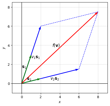
5. Column picture#
Let \(A\in\mathbb{R}^{2\times 2}\) with columns \(\mathbf{s}_1,\mathbf{s}_2\):
For \(\mathbf{v}=\begin{bmatrix}v_1\\v_2\end{bmatrix}\),
This means: the image consists of all linear combinations of the columns of \(A\).
Geometric consequence in \(\mathbb{R}^2\)
If \(\mathbf{s}_1=\mathbf{0}\) and \(\mathbf{s}_2=\mathbf{0}\), then the image is just the point \((0,0)\).
If \(\mathbf{s}_1,\mathbf{s}_2\) are nonzero but parallel, the image is a line through the origin.
If \(\mathbf{s}_1,\mathbf{s}_2\) are not parallel, the image is all of \(\mathbb{R}^2\).
The following code cell visualizes the decomposition \(A\mathbf{v}=v_1\mathbf{s}_1+v_2\mathbf{s}_2\):
# --- input (experiment with the numerical values here) ---
s1 = np.array([1, 3])      # first column
s2 = np.array([2, 0.5])    # second column
v1, v2 = 2, 3              # coefficients
# ------------------------------------------

f_v = v1*s1 + v2*s2

fig, ax = plt.subplots()

# draw column products
ax.quiver(0, 0, *v1*s1, angles='xy', scale_units='xy', scale=1, color="blue")
ax.text(*v1*s1/2, r'$v_1\mathbf{s}_1$', fontsize=12, color="k", ha='left', va='top')
ax.plot([v1*s1[0], f_v[0]], [v1*s1[1], f_v[1]], 'b--', linewidth=1)

ax.quiver(0, 0, *v2*s2, angles='xy', scale_units='xy', scale=1, color="blue")
ax.text(*v2*s2/2, r'$v_2\mathbf{s}_2$', fontsize=12, color="k", ha='left', va='top')
ax.plot([v2*s2[0], f_v[0]], [v2*s2[1], f_v[1]], 'b--', linewidth=1)

# draw columns
ax.quiver(0, 0, *s1, angles='xy', scale_units='xy', scale=1, color="green")
ax.text(*s1/2, r'$\mathbf{s}_1$', fontsize=12, color="k", ha='right', va='bottom')
ax.quiver(0, 0, *s2, angles='xy', scale_units='xy', scale=1, color="green")
ax.text(*s2/2, r'$\mathbf{s}_2$', fontsize=12, color="k", ha='right', va='bottom')

# draw f(v)
ax.quiver(0, 0, *f_v, angles='xy', scale_units='xy', scale=1, color="r")
ax.text(*f_v/2, r'$f(\mathbf{v})$', fontsize=12, color="k", ha='right', va='bottom')

# plot appearance
ax.axhline(0, color="black", linewidth=1)
ax.axvline(0, color="black", linewidth=1)
ax.set_aspect("equal")
ax.set_xlim(min(v1*s1[0], v2*s2[0], f_v[0], 0) - 1, max(v1*s1[0], v2*s2[0], f_v[0], 0) + 1)
ax.set_ylim(min(v1*s1[1], v2*s2[1], f_v[1], 0) - 1, max(v1*s1[1], v2*s2[1], f_v[1], 0) + 1)
ax.grid(True, which='both', linestyle='--', linewidth=0.5)
ax.set_xlabel("$x$")
ax.set_ylabel("$y$")
plt.show()
6. Rank and invertibility#
The rank of a matrix \(A\) is the dimension of the space spanned by its columns (equivalently: the number of linearly independent columns).
In \(\mathbb{R}^{2\times 2}\), rank can be \(0\), \(1\), or \(2\).
If \(\mathrm{rank}(A)=2\), the columns are not parallel, the image is all of \(\mathbb{R}^2\), and \(A\) is invertible.
If \(\mathrm{rank}(A)<2\), the transformation “collapses” space into a line or a point, and \(A\) is not invertible.
In Python, you can compute rank via:
# Example:
A = np.array([[1, 1], [-1, 1]])
print(np.linalg.matrix_rank(A))
2
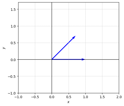
7. Rotations#
A rotation by an angle \(\theta\) (radians) in the positive direction is given by
Then \(R(\theta)\mathbf{v}\) is \(\mathbf{v}\) rotated by \(\theta\), and importantly the length is preserved:
Rotation matrices are special
Rotation matrices are orthogonal and satisfy \(R(\theta)^{-1}=R(\theta)^\top = R(-\theta)\).
So the inverse rotation is just “rotate back”.
A simple visualization:
def draw_vectors(vector_list):
    fig, ax = plt.subplots()
    for v in vector_list:
        ax.quiver(0, 0, *v, angles='xy', scale_units='xy', scale=1, color="blue")
    all_x = [v[0] for v in vector_list] + [0]
    all_y = [v[1] for v in vector_list] + [0]
    ax.set_xlim(min(all_x) - 1, max(all_x) + 1)
    ax.set_ylim(min(all_y) - 1, max(all_y) + 1)
    ax.axhline(0, color="black", linewidth=1)
    ax.axvline(0, color="black", linewidth=1)
    ax.set_aspect("equal")
    ax.grid(True, which='both', linestyle='--', linewidth=0.5)
    ax.set_xlabel("$x$")
    ax.set_ylabel("$y$")
    plt.show()

e1 = np.array([1,0])
theta = np.pi/4
R = np.array([[np.cos(theta), -np.sin(theta)],
              [np.sin(theta),  np.cos(theta)]])
draw_vectors([e1, R @ e1])
8. Matrix–matrix products and composition of transformations#
If \(M\in\mathbb{R}^{m\times n}\) and \(N\in\mathbb{R}^{n\times k}\), the product \(MN\) is an \(m\times k\) matrix.
The key interpretation is composition:
So multiplying matrices corresponds to applying linear maps one after the other.
Order matters
In general \(MN\neq NM\).
So the order of applying transformations matters (rotate then scale is not necessarily the same as scale then rotate).
9. Inverse matrices#
A square matrix \(A\in\mathbb{R}^{n\times n}\) is invertible if there exists a matrix \(A^{-1}\) such that
where \(I\) is the identity matrix.
For a rotation matrix \(R(\theta)\),
10. Diagonal matrices: scaling and coordinate-wise effects#
A diagonal matrix has the form
Then
So diagonal matrices scale the \(x\)- and \(y\)-coordinates separately.
Invertibility of diagonal matrices
A diagonal matrix is invertible exactly when all diagonal entries are nonzero.
Then \(D^{-1}=\mathrm{diag}(1/d_1, 1/d_2)\).
11. Change of coordinates (rotating the coordinate system)#
Suppose you have an \(x\)-\(y\) coordinate system and a rotated \(x'\)-\(y'\) system (rotated by \(\theta\)).
If a vector has coordinates \((x',y')\) in the rotated system, then its coordinates \((x,y)\) in the original system satisfy:
Conversely,
This is the same idea as “rotating the axes” versus “rotating the vector”: one is the inverse of the other.
Practical takeaway
A change of coordinates is just multiplying by the appropriate matrix (often a rotation matrix or its inverse).
It is the same linear algebra, just a different interpretation.