Self-Driving Cars

Self-Driving Cars#

About the project#

Duration: 20–50 hours (including typesetting final report in LaTeX)
Prerequisites: Differential equations (1st/2nd order linear ODEs), linear algebra (matrices, eigenvalues/diagonalization), stability and complex eigenvalues, basic calculus, basic Python programming (NumPy/matplotlib)
Python packages: NumPy, matplotlib, sympy, scipy
Learning objectives: Model car-following dynamics with ODEs, analyze homogeneous/forced linear ODEs via characteristic polynomials, derive particular solutions by variation of parameters, study propagation of disturbances in a convoy, set up block-matrix ODE systems on a ring, and relate stability of stationary solutions to eigenvalues

Important

This project was created by Kristian Uldall Kristiansen, DTU Compute.

Background#

In this project you will look at a simple model for self-driving cars in a line, see Figure 1, defined as follows.

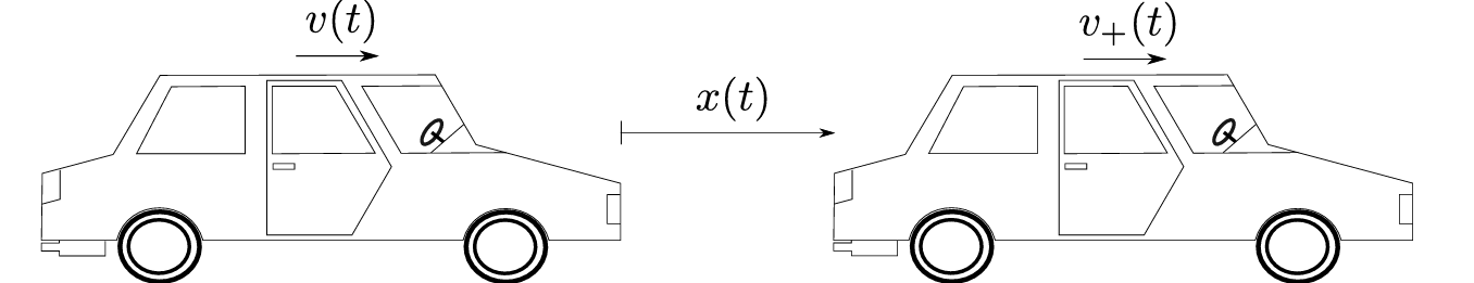
Figure 1: Self-driving cars. (In the analysis we do not account for the cars’ physical size and therefore represent them as points.)

The acceleration of a car in the line, with speed $v(t)$ (measured in $\mathrm{m\,s^{-1}}$) and distance to the car in front $x(t)$ (measured in $\mathrm{m}$), is given by

\[ a(t)=b\,(v_+(t)-v(t))+c\,(x(t)-x_*(t)), \qquad \text{(1)} \]

measured in $\mathrm{m\,s^{-2}}$. Here $t$ denotes time (measured in $\mathrm{s}$), $b$ and $c$ are parameters (with units $\mathrm{s^{-1}}$ and $\mathrm{s^{-2}}$, respectively), $v_+(t)>0$ is the speed of the car in front, and $x_*(t)>0$ is a desired distance to the car in front. We assume that

\[ x_*(t)=T\,v_+(t), \qquad \text{(2)} \]

where $T$ is a new parameter (with unit $\mathrm{s}$).

Assumption
We do not account for the cars’ physical size and will think of them as points.

Exercise 1
First argue that $T>0$. Next, we emphasize that the idea of the model is that the car (via its motor and braking system) should follow the acceleration in (1) and thereby drive the speed $v(t)$ and the relative distance $x(t)$ toward $v_+(t)$ and $x_*(t)$, respectively.
With this in mind, consider Figure 2 and state the desired sign of $a(t)$ in quadrants $K_2$ and $K_4$ in the $(x,v)$-plane (and optionally also along the red and blue lines). What does this imply for the signs of $b$ and $c$?

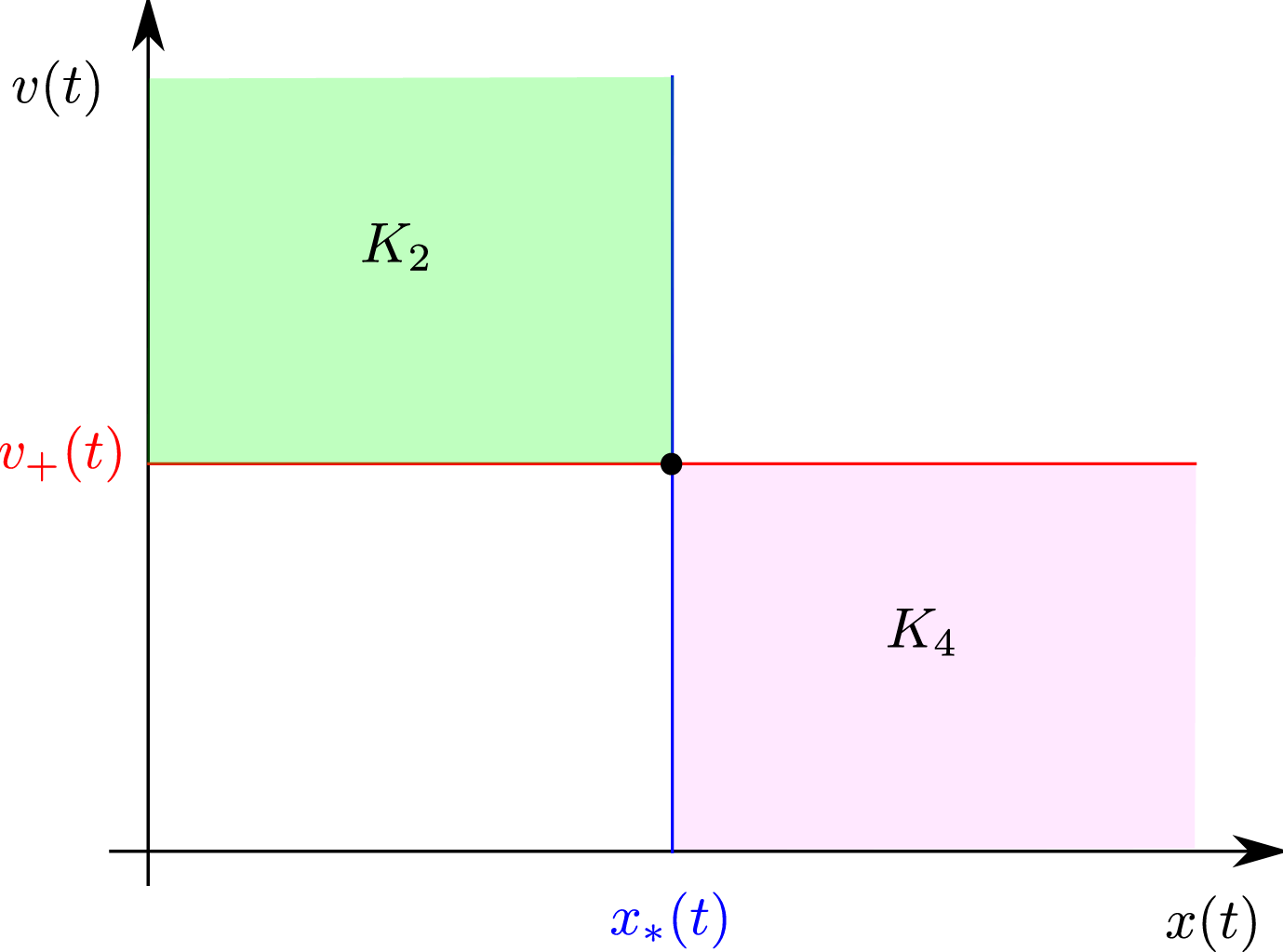
Figure 2: The quadrants $K_2$ and $K_4$ relevant for Exercise 1.

We now assume that $v_+=v_+(t)$, $t\in\mathbb{R}$, is a known differentiable function.

Exercise 2
Show that the relative distance $x(t)$ satisfies a second-order linear differential equation of the form

\[\begin{equation*} x''(t)+b\,x'(t)+c\,x(t)=F(t), \qquad \text{(3)} \end{equation*}\]

and that

\[\begin{equation*} v(t)=v_+(t)-x'(t). \end{equation*}\]

Determine the function $F$, expressed using the constants $c,T$ and the function $v_+(t)$.

Assumption
From here on, you may assume

\[\begin{equation*} c=1. \qquad \text{(4)} \end{equation*}\]

One can show that this is without loss of generality.

Consider the characteristic polynomial

\[ P(\lambda)=\lambda^2+b\lambda+c. \qquad \text{(5)} \]

Exercise 3
(a) Determine the complete real solution to the homogeneous equation corresponding to (3). It will be necessary to split the analysis into three cases $b<b_{cr}$, $b=b_{cr}$, $b>b_{cr}$, where $b_{cr}>0$ must be determined and characterized.
(b) Given your conditions on $b,c$ and $T$ from Exercise 1, what can you say about any solution $x(t)$, $t\in\mathbb{R}$, to the homogeneous system as $t o\infty$?

In your answer to Exercise 3, two arbitrary constants $c_1,c_2\in\mathbb{R}$ will appear. We call these constants integration constants. They can be determined from initial conditions $x(0)=x_0$, $x'(0)=x_1$ with given $x_0,x_1$.

Exercise 4
Consider (3) with $F:\mathbb{R} o\mathbb{R}$ a known continuous function and first assume that $\lambda_1$ and $\lambda_2$ are two simple roots of $P$, $\lambda_1 eq \lambda_2$. Show that

\[\begin{equation*} x^p(t)=\frac{1}{\lambda_1-\lambda_2}\left( e^{\lambda_1 t}\int_0^t F(s)e^{-\lambda_1 s}\,ds -e^{\lambda_2 t}\int_0^t F(s)e^{-\lambda_2 s}\,ds \right), \qquad t\in\mathbb{R}, \qquad \text{(6)} \end{equation*}\]

is a particular solution to (3), and that $x^p(t)$, $t\in\mathbb{R}$, is real. Include intermediate steps to a reasonable extent!

Hint: What does it mean that $x^p$ is a particular solution? For the fact that $x^p$ is real, show that $x^p(t)=\overline{x^p(t)}$ for all $t\in\mathbb{R}$. You may use that $b,c$ and $F(t)$ are real for all $t\in\mathbb{R}$, and the following conjugation rules:

$\overline{(z_1 z_2)}=\overline z_1\,\overline z_2$, in particular $\overline{(z_1^{-1})}=\overline z_1^{-1}$.

$\overline{z_1\pm z_2}=\overline z_1\pm \overline z_2$.

$\overline{e^{z_1}}=e^{\overline z_1}$.

$\overline{\int_0^t f(s)\,ds}=\int_0^t \overline{f(s)}\,ds$, $t\in\mathbb{R}$,

for all complex numbers $z_1,z_2\in\mathbb{C}$ and all $f:\mathbb{R}\to\mathbb{C}$. (Note: These rules are not included in the Mat1a notes.)

Exercise 5
Consider again (3) with $F:\mathbb{R}\to\mathbb{R}$ a known continuous function and assume that $\lambda_1$ is a double root. Show that

\[\begin{equation*} x^p(t)=t e^{\lambda_1 t}\int_0^t F(s)e^{-\lambda_1 s}\,ds -e^{\lambda_1 t}\int_0^t F(s)s e^{-\lambda_1 s}\,ds, \qquad t\in\mathbb{R}, \qquad \text{(7)} \end{equation*}\]

is a particular solution to (3). Why is $x^p(t)$ real for all $t\in\mathbb{R}$? Include intermediate steps to a reasonable extent!

Exercise 6
Show that $x^p(0)=0$ and $(x^p)'(0)=0$. You may restrict to the case where $P$ has two simple roots $\lambda_1$ and $\lambda_2$, $\lambda_1\ne\lambda_2$.

Exercise 7
Write down the complete real solution to (3). Assume again that $F:\mathbb{R}\to\mathbb{R}$ is a known continuous function.

A convoy of cars#

We now consider an infinite convoy of cars with a leading car (which we call $j=0$) that drives with a known speed $v_0(t)>0$, $t\in\mathbb{R}$. The following cars are numbered by $j\in\mathbb{N}$, such that for all $j\in\mathbb{N}$:

$x_j(t)$ denotes the distance between car $j-1$ and car $j$.
$v_j(t)$ denotes the speed of car $j$.
The acceleration $a_j(t)$ of car $j$ is given by (1) in the form $$ a_j(t)=b\,(v_{j-1}(t)-v_j(t))+c\,(x_j(t)-T v_{j-1}(t)). $$

See Figure 3.

Figure 3: A convoy of self-driving cars. (In the analysis we do not account for the cars’ physical size and therefore represent them as points.)

Exercise 8
Show that

\[\begin{equation*} \begin{cases} x_j''(t)+b\,x_j'(t)+c\,x_j(t)=v_{j-1}'(t)+cT\,v_{j-1}(t),\\ v_j(t)=v_{j-1}(t)-x_j'(t), \end{cases} \qquad \text{for all } j\in\mathbb{N}. \qquad \text{(8)} \end{equation*}\]

We now assume that $v_0(t)$, $t\in\mathbb{R}$, is constant (which we denote by $v_0>0$).

Exercise 9
Show that $x_j(t)=T v_0$ and $v_j(t)=v_0$ for all $t\in\mathbb{R}$ and all $j\in\mathbb{N}$ is a solution to (8).

We call the solution in Exercise 9 a stationary solution.

The model has its obvious limitations. For example, it does not enforce that $x_j(t)$ and $v_j(t)$ are strictly positive. The idea is that it can be relevant (for some parameter values) when considering “small” deviations from the stationary solution.

We therefore consider an initial value problem defined by (8) and the initial conditions

\[\begin{split} x_j(0)=T v_0, \qquad x_j'(0)= \begin{cases} y_1, & j=1,\\ 0, & j\in\mathbb{N}\setminus\{1\}, \end{cases} \qquad \text{(9)} \end{split}\]

where $0<y_1<v_0$, for all $j\in\mathbb{N}$. Note that

\[\begin{split} v_j(0)= \begin{cases} v_0-y_1, & j=1,\\ v_0, & j\in\mathbb{N}\setminus\{1\}. \end{cases} \end{split}\]

Exercise 10
(a) First give an interpretation of these initial conditions.
(b) Next consider

\[\begin{equation*} v_0=20, \quad y_1=1, \quad c=1, \quad T=\frac{1}{10}, \quad b=2, \qquad \text{(10)} \end{equation*}\]

and compute (for these parameter values) the solutions $x_1(t)$ and $v_1(t)$ for $t\ge 0$ using your answer to Exercise 7. Use the initial conditions in (9) with $j=1$ to determine the integration constants. It may also be helpful to use Exercise 6.
(c) Then determine $x_2(t),v_2(t)$ and $x_3(t),v_3(t)$ by using (8) and (9) with $j=2$ and $j=3$ (again for the parameter values in (10)).
(d) Plot the graphs of the functions you found for $t\ge 0$ and comment on the result.
(e) Investigate whether $x_1(t),x_2(t),x_3(t)$ (and $v_1(t),v_2(t),v_3(t)$) converge to $T v_0=2$ (and $v_0=20$, respectively), corresponding to the stationary solution, as $t\to\infty$.

We will now write an algorithm to compute the solutions $x_j(t)$ and $v_j(t)$, $t\in\mathbb{R}$, $j\in\mathbb{N}$, to (8) and (9) recursively. In your answer to the next exercise, you may assume that the roots $\lambda_1$ and $\lambda_2$ of $P$ are simple, $\lambda_1\ne\lambda_2$.

Exercise 11
(a) Start by solving for $x_1(t),v_1(t)$, $t\in\mathbb{R}$. Your expressions must be free of integration constants; therefore use the initial conditions (and Exercise 6) to solve for the integration constants $c_1$ and $c_2$ (as functions of $v_0$ and $y_1$) in your general solution formulas from Exercise 7.
(b) Then describe a function that takes $x_{j-1}(t),v_{j-1}(t)$, $t\in\mathbb{R}$, with $j\in\mathbb{N}$, $j\ge 2$, as input and returns $x_j(t),v_j(t)$, $t\in\mathbb{R}$, as output. The answer must again be free of integration constants (using the initial conditions for $x_j(0)$ and $x_j'(0)$ for $j\ge 2$).

Exercise 12
(a) Assume $v_0=20$, $y_1=1$, $c=1$, $T=\frac{1}{10}$, and investigate the solution to the initial value problem given by (8) and (9) for different values of $b$. In Mathematics 1b you have used the trapezoidal rule for numerical integration. Here you should extend it to a cumulative trapezoidal rule on a fixed time grid so you can evaluate the integrals in the particular solution by updating the running trapezoid sum and thereby iterate the system numerically for $j=1,2,\dots$.
(b) If possible, determine the smallest $j\in\mathbb{N}$ such that there exists $t>0$ with $x_j(t)<0$ or $v_j(t)<0$. Start for example with $b=\frac{3}{2}$, $b=2$, and $b=\frac{5}{2}$. This can be computationally heavy, so only consider $j\lesssim 70$ and $0\le t\le 100$.
(c) Discuss the result.

Cars on a ring#

In the remaining part of the project, we consider $N\in\mathbb{N}$, $N\ge 2$, cars on a ring driving counterclockwise. We number the cars like on a clock: starting at 12 o’clock and moving clockwise, we label the first car we meet as $j=1$, then $j=2$, and so on up to $j=N$, see Figure 4. In this way we have numbered all $N$ cars, but if we continue around past 12 o’clock again we meet car $j=N+1$, which is car $j=1$ again. We can continue this way, and thus identify car number $j=k$ (for $k\in\mathbb{N}$, $1\le k\le N$) with all indices $j=k+nN$ for all $n\in\mathbb{Z}$. Here $n$ indicates how many times (with sign) we have moved around the ring. If $n<0$, then we have moved $-n\in\mathbb{N}$ times around counterclockwise.

As before, $v_j(t)$ denotes the speed of car $j$, while $x_j(t)$ denotes the (along-the-ring) distance between car $j-1$ and car $j$.

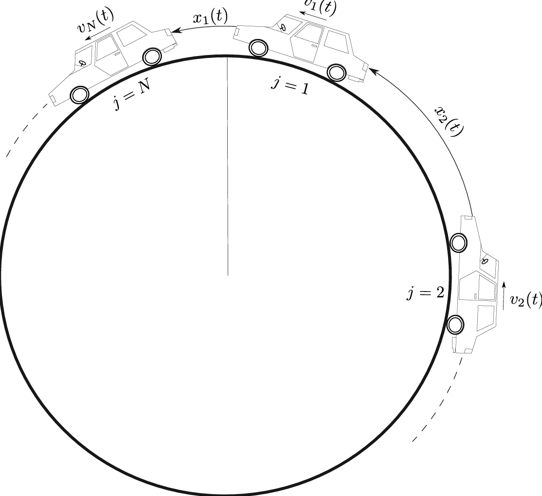
Figure 4: Self-driving cars on a ring. (In the analysis we do not account for the cars’ physical size and therefore represent them as points.)

Exercise 13
Explain the claim: $v_j=v_{j+nN}$ and $x_j=x_{j+nN}$ for all $n\in\mathbb{Z}$.

We assume (again) that the acceleration of car $j$ is given by

\[ a_j(t)=b\,(v_{j-1}(t)-v_j(t))+c\,(x_j(t)-T v_{j-1}(t)). \]

Exercise 14
Define the vector function

\[\begin{equation*} \mathbf z_j(t)= \begin{pmatrix} x_j(t)\\ v_j(t) \end{pmatrix}\in\mathbb{R}^2, \qquad t\in\mathbb{R}, \end{equation*}\]

for all $j\in\mathbb{Z}$. Determine $\mathbf A\in\mathbb{R}^{2\times 2}$ and $\mathbf B\in\mathbb{R}^{2\times 2}$ such that

\[\begin{equation*} \mathbf z_j'(t)=\mathbf A\,\mathbf z_j(t)+\mathbf B\,\mathbf z_{j-1}(t), \qquad \text{for all } j\in\mathbb{Z}, \qquad \text{(11)} \end{equation*}\]

and in particular

\[\begin{equation*} \mathbf z_1'(t)=\mathbf A\,\mathbf z_1(t)+\mathbf B\,\mathbf z_N(t). \qquad \text{(12)} \end{equation*}\]

Exercise 15
Define

\[\begin{equation*} \mathbf z(t)= \begin{pmatrix} \mathbf z_1(t)\\ \mathbf z_2(t)\\ \vdots\\ \mathbf z_N(t) \end{pmatrix}\in\mathbb{R}^{2N}, \qquad t\in\mathbb{R}. \end{equation*}\]

Show that

\[\begin{equation*} \mathbf z'(t)=\mathbf C\,\mathbf z(t), \qquad \text{(13)} \end{equation*}\]

where $\mathbf C\in\mathbb{R}^{2N\times 2N}$. It may be helpful to build $\mathbf C$ from $2\times 2$ blocks $\mathbf C_{i,j}\in\mathbb{R}^{2\times 2}$, $i,j=1,\dots,N$, and determine all $\mathbf C_{i,j}$ that are different from the zero matrix.

Exercise 16
Show that

\[\begin{equation*} \mathbf w_1= \begin{pmatrix} 1\\ T^{-1} \end{pmatrix} \end{equation*}\]

spans $\ker(\mathbf A+\mathbf B)$. Then define

\[\begin{equation*} \mathbf v_1= \begin{pmatrix} \mathbf w_1\\ \vdots\\ \mathbf w_1 \end{pmatrix}, \qquad \text{(14)} \end{equation*}\]

and show that $\mathbf v_1\in\ker(\mathbf C)$.

Exercise 17
Argue that

\[\begin{equation*} \mathbf z(t)=c_1\,\mathbf v_1, \qquad t\in\mathbb{R}, \qquad \text{(15)} \end{equation*}\]

is a solution to (13) for all $c_1\in\mathbb{R}$.

We say that a solution $\mathbf z(t)$ has ring length $R>0$ if

\[ R:=x_1(t)+\cdots+x_N(t). \]

Exercise 18
Give an interpretation and show that $R$ is constant.
Hint: First show that $x_1'(t)+\cdots+x_i'(t)=v_N(t)-v_i(t)$ for all $i\in\mathbb{N}$ by induction. Use $i=1$: $x_1'(t)=v_N(t)-v_1(t)$ as the induction start.

Exercise 19
Determine the constant $c_1=c_1(R)$ such that (15) has ring length $R$.

The solution in (15) with $c_1=c_1(R)$ is again called the stationary solution (with ring length $R>0$). As in the convoy case, it is the desired state of the system. We are therefore interested in stability of the stationary solutions, in particular finding parameters such that the stationary solution (15) is stable (preferably for all $N$).

We understand stability as follows:

Definition (asymptotic stability). The stationary solution with ring length $R>0$ is asymptotically stable if the following holds for all solutions $\mathbf z(t)$, $t\in\mathbb{R}$, of (13) with ring length $R>0$:

\[ \lVert \mathbf z(t)-c_1(R)\mathbf v_1\rVert\to 0 \quad \text{as } t\to\infty. \]

On the other hand, if there exists a solution $\mathbf z(t)$ with ring length $R>0$ such that

\[ \lVert \mathbf z(t)-c_1(R)\mathbf v_1\rVert\to \infty \quad \text{as } t\to\infty, \]

then the stationary solution is called unstable.

Remark (background). There is a third possibility, where $\mathbf z(t)-c_1(R)\mathbf v_1$ neither grows unboundedly nor goes to zero as $t\to\infty$, but is merely bounded for all solutions with ring length $R$ and all $t\ge 0$. One could call this “marginal stability”, but we will not worry about this case in the project.

We will use the following theorem (without proof):

Theorem A. Let $\lambda_1=0,\lambda_2,\dots,\lambda_{2N}\in\mathbb{C}$ denote the eigenvalues of $\mathbf C$ (with multiplicity). Then:

The stationary solution is asymptotically stable if and only if $$ \operatorname{Re}(\lambda_i)<0 \quad \text{for all } i=2,\dots,2N. \qquad \text{(16)} $$
If there exists an eigenvalue $\lambda_i$ with $\operatorname{Re}(\lambda_i)>0$ for some $i\in\{2,\dots,2N\}$, then the stationary solution is unstable.

Remark. Stability is independent of the ring length $R$.

Exercise 20
Use Chapter 12 of the Mat1b textbook to show that condition (16) is sufficient for asymptotic stability (part (i) of Theorem A). In your answer, you may assume that $\mathbf C$ can be diagonalized with eigenvalues $\lambda_1=0,\lambda_2,\dots,\lambda_{2N}$ and $2N$ corresponding linearly independent eigenvectors $\mathbf v_1,\dots,\mathbf v_{2N}$.

We now try to determine the remaining eigenvalues $\lambda_2,\dots,\lambda_{2N}\in\mathbb{C}$ (with multiplicity) of $\mathbf C$.

Let $\omega\in\mathbb{C}$ satisfy

\[ \omega^N=1. \qquad \text{(17)} \]

Exercise 21
Show that all solutions to (17) can be written in the form

\[\begin{equation*} \omega=e^{i\theta}, \qquad \theta=\frac{2\pi n}{N},\ n=0,\dots,N-1. \qquad \text{(18)} \end{equation*}\]

Exercise 22
Determine $\mathbf D=\mathbf D(\omega)\in\mathbb{C}^{2\times 2}$ such that

\[\begin{equation*} \mathbf v= \begin{pmatrix} \omega^{N-1}\mathbf w\\ \omega^{N-2}\mathbf w\\ \vdots\\ \omega^{N-j}\mathbf w\\ \vdots\\ \mathbf w \end{pmatrix}, \qquad \mathbf w\in\mathbb{C}^2, \qquad \text{(19)} \end{equation*}\]

is an eigenvector of $\mathbf C$ with eigenvalue $\lambda$ if and only if

\[\begin{equation*} \mathbf D\,\mathbf w=\lambda\,\mathbf w. \end{equation*}\]

Hint: Use the block structure of $\mathbf C$ from Exercise 15.

We now consider first the case $\omega=1$.

Exercise 23
Show that $\lambda_1=0$ and $\lambda_2=-cT$ are the eigenvalues of $\mathbf D(1)$. Determine the corresponding eigenvectors $\mathbf w_1$ and $\mathbf w_2$ and compare $\mathbf w_1$ with your answer in Exercise 16.

Exercise 24
Determine the eigenvalues $\Lambda_1(\theta)$ and $\Lambda_2(\theta)$ of $\mathbf D(e^{i\theta})$. Choose $\Lambda_1(\theta)$ such that $\Lambda_1(0)=\lambda_1=0$ and $\Lambda_2(0)=\lambda_2=-cT$.

We can now reach the following conclusion:

Theorem B. The eigenvalues of $\mathbf C$ can be listed as $\lambda_1=0,\lambda_2=-cT,\lambda_3,\dots,\lambda_{2N}\in\mathbb{C}$ (with multiplicity), where $\lambda_1=0$ and $\lambda_2=-cT$ arise from $\theta=0$ as in Exercise 23. The remaining eigenvalues $\lambda_3,\dots,\lambda_{2N}$ are given by the expressions $\Lambda_1(\theta)$ and $\Lambda_2(\theta)$ for the $N-1$ distinct values $\theta=\frac{2\pi n}{N}$, $n=1,\dots,N-1$ (i.e. $\theta\ne 0$).

Exercise 25
(a) Investigate asymptotic stability (e.g. in SymPy) using plots of $\operatorname{Re}(\Lambda_1(\theta))$ and $\operatorname{Re}(\Lambda_2(\theta))$ as functions of $\theta\in[0,2\pi]$ for $c=1$, $T=1$, and three different values of $b$: $b=1$, $b=\frac{3}{2}$, and $b=2$.
(b) In particular, if you find a $\theta$ such that $\operatorname{Re}(\Lambda_i(\theta))>0$ for $i=1$ or $i=2$, determine (if possible) a critical value $N_{cr}$ such that the system is unstable for all $N>N_{cr}$ and asymptotically stable for all $N<N_{cr}$.

We now determine a sharpened necessary condition for stability (for all $N$).

Exercise 26
(a) Let $\Lambda_1(\theta)\in\mathbb{C}$, $\theta\in\mathbb{R}$, denote the eigenvalue of $\mathbf D(e^{i\theta})$ from Exercise 24 with $\Lambda_1(0)=0$. Determine the degree-2 Taylor polynomial $P_2(\theta)$ for $\Lambda_1(\theta)$ around $\theta=0$ (see Definition 4.2.1 in the Mat1b textbook).
(b) Determine $b_{cr,new}$ such that $\operatorname{Re}P_2(\theta)<0$ for all $\theta\ne 0$ if and only if

\[\begin{equation*} b>b_{cr,new}. \qquad \text{(20)} \end{equation*}\]

Exercise 27
Investigate (numerically) whether (20) is a sufficient condition for asymptotic stability for all $N\in\mathbb{N}$.