Optical Waveguides#
Modes, nonlinearities, and quantum optics#
About the project#
Duration: 20–50 hours (including typesetting final report in LaTeX)
Prerequisites: Multivariable calculus (grad/div/curl, vector identities), PDEs (wave equation, Helmholtz equation), ODEs (boundary value problems), basic complex numbers, basic Python programming; familiarity with Bessel functions is helpful
Python packages: NumPy, matplotlib, sympy, scipy
Learning objectives: Derive the wave and Helmholtz equations from Maxwell’s equations, analyze guided modes in planar and cylindrical waveguides, work with Bessel-function boundary conditions, compute dispersion/effective index, and model photon-pair generation and spectral correlations in fiber-based quantum optics
Background#
Since the first demonstrations of data transmission through optical fibers, these fibers have formed the backbone of the modern communications infrastructure. In 2019 it was assumed that global internet traffic exceeded 100 exabit per second (\(10^{18}\) bit/s). This traffic is sent through thousands of kilometers of optical fibers. Besides their impressive ability to transport data, modern optical fibers—and other forms of waveguides—also have many other applications. For example, fibers are a central part of critical network components such as amplifiers and can be used in sensors, lasers, and more.
In this project assignment you will investigate how light behaves when it is confined to the very small core (typically under 10 micrometers) of an optical fiber. After a short introduction to electromagnetism in Part 1, you will in Part 2 explore how this confinement gives rise to discrete modes, analogous to the standing waves that arise when sound is confined to a guitar string of fixed length. These modes have different properties, for example their spatial distribution of light in the core and their propagation speed through the fiber. Part 3 concerns the generation of single photons in pairs. These photon pairs can, for instance, be used as part of an optical quantum computer, and you will among other things investigate how the photons’ quantum-mechanical properties depend on the properties of the optical fiber. Each photon pair is generated using a special nonlinear process in waveguides, called four-wave mixing, which can be used to create optical fields at wavelengths different from the light you send into the fiber.
Part 1 – Basic electromagnetism#
Maxwell’s equations#
Light is electromagnetic waves, and working with light therefore requires some knowledge of basic electromagnetism. Electromagnetism describes the behavior of the electric field \(E\) and the magnetic field \(B\). These two vector fields can vary in both space and time and are described by a set of four partial differential equations, called Maxwell’s equations, which (in situations without so-called external charges or currents) take the form:
Here \(\mu_0 = 4\pi\times 10^{-7}\ \mathrm{V\,s/(A\,m)}\) is the so-called vacuum permeability and \(\epsilon\) is the permittivity, which in vacuum has the value \(\epsilon_0 = 8.82\times 10^{-12}\ \mathrm{C/(m\,V)}\), but has a different value in other materials such as glass. Moreover, it can vary in space as \(\epsilon(x,y,z)\). If one deals with a material (i.e. not vacuum), one typically writes \(\epsilon = \epsilon_0\epsilon_r\), where \(\epsilon_r\) is called the relative permittivity. Materials are also often described through their refractive index \(n\), given by \(n^2 = \epsilon_r\). A difference between two materials’ refractive indices dictates how light is deflected when it meets the interface between one material and the other, and this is central to how one guides light in an optical fiber.
In rectangular coordinates the \(\nabla\) operator is, as you know,
where hats indicate unit vectors. This gives rise to the familiar expressions for the gradient of scalar fields and the divergence and curl of vector fields.
Exercise 1
Show, using the vector identity \(\nabla\times(\nabla\times A)=\nabla(\nabla\cdot A)-\nabla^2A\), that these equations can be combined into a partial differential equation involving only the magnetic field \(B\):\[\begin{equation*} \nabla^2 B - \mu_0\epsilon\,\frac{\partial^2 B}{\partial t^2}=0.\tag{3} \end{equation*}\]Here \(\nabla^2\) is the vector Laplace operator.
Hint: Start with the equation for the curl of \(B\) and use the stated vector identity.
Equation (3) is called the wave equation and arises in extremely many places in physics. In rectangular coordinates, the vector Laplace operator takes the form
where \(A_x, A_y\) and \(A_z\) are the components of \(A\).
Exercise 2
Show that all twice-differentiable vector functions of one variable of the form \(A(z-vt)\) are solutions to the wave equation. Explain why we call this a wave traveling in the positive \(z\) direction, with speed \(v\). Find an expression for \(v\) in terms of the electromagnetic constants and compute its value in vacuum. Do you recognize the number?
In the rest of the assignment we restrict ourselves to monochromatic light, i.e. light with a single wavelength. The magnetic field therefore has the form \(B = F\exp(-i\omega t)\), where \(F\) is a vector function that depends only on the spatial coordinates and \(\omega\) is the angular frequency, which relates directly to the wavelength \(\lambda\) through \(\omega = 2\pi c/\lambda\), where \(c\) is the speed of light in vacuum.
Exercise 3
Show that this ansatz leads to the Helmholtz equation\[\begin{equation*} \nabla^2 F + n^2 k^2 F = 0.\tag{5} \end{equation*}\]where \(n=c/v\) is the refractive index. Determine the vacuum wavenumber \(k\) in terms of the other variables.
When the refractive index \(n\) does not change too rapidly with respect to the spatial coordinates, one can to a good approximation consider only a single component of either the electric or magnetic field. We call this component \(\Psi\), which then satisfies the scalar Helmholtz equation
together with the requirement that \(\Psi\) and its first derivative are continuous everywhere in space.
Exercise 4
Show that the scalar Laplace operator, defined as the divergence of the gradient in rectangular coordinates, is given by\[\begin{equation*} \nabla^2\Psi = \frac{\partial^2\Psi}{\partial x^2}+\frac{\partial^2\Psi}{\partial y^2}+\frac{\partial^2\Psi}{\partial z^2}.\tag{7} \end{equation*}\]
When you later work with the field in an optical fiber, you can exploit the system’s symmetry better by working in cylindrical coordinates, as illustrated in Figure 1. They are related to the usual rectangular coordinates \(x,y,z\) as follows:
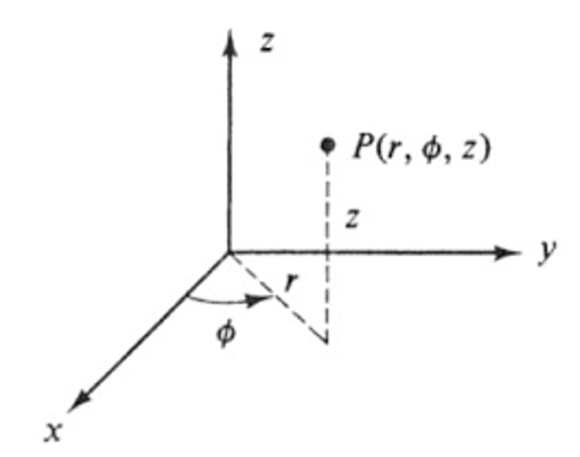
Figure 1 – The relationship between the usual rectangular coordinates and the cylindrical coordinates.
To solve the Helmholtz equation in a cylindrical coordinate system, we must find an expression for the Laplace operator in cylindrical coordinates.
Exercise 5
Use the chain rule to show that\[\begin{equation*} \frac{\partial}{\partial x}=-\frac{\sin\varphi}{r}\frac{\partial}{\partial\varphi}+\cos\varphi\frac{\partial}{\partial r},\tag{11} \end{equation*}\]\[\begin{equation*} \frac{\partial}{\partial y}=\frac{\cos\varphi}{r}\frac{\partial}{\partial\varphi}+\sin\varphi\frac{\partial}{\partial r}.\tag{12} \end{equation*}\]Hint: It may be easier to see by inserting the helper function \(f(\varphi,r)\) into the identity.
Exercise 6
Use the result from the previous exercise to show that the scalar Laplace operator can be expressed as follows in cylindrical coordinates:\[\begin{equation*} \nabla^2 = \frac{\partial^2}{\partial r^2} +\frac{1}{r}\frac{\partial}{\partial r} +\frac{1}{r^2}\frac{\partial^2}{\partial\varphi^2} +\frac{\partial^2}{\partial z^2}. \tag{13} \end{equation*}\]
Part 2 – Optical waveguides#
As discussed in the previous part, the optical field \(\Psi\) in a waveguide is approximately described by the scalar Helmholtz equation
where \(k\) is the vacuum wavenumber and \(n\) is the refractive index. Across changes in refractive index, both \(\Psi\) and its first derivative must be continuous across the transition between two materials, each with its own refractive index.
Planar waveguide#
We first consider a planar waveguide, as shown in Figure 2. The waveguide is infinitely long in the \(y\) and \(z\) directions, but consists of a homogeneous material of height \(H\) and refractive index \(n\) between two perfectly conducting layers, which means that \(\Psi=0\) in these layers.
We guess that the field in the waveguide can be described by the form \(\Psi(x,y,z)=X(x)\exp(i\beta z)\), where \(\beta\) is the so-called propagation constant, which is currently unknown.
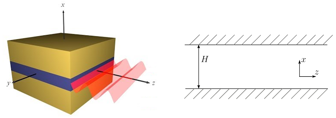
Figure 2 – 3D figure and cross section of the planar waveguide, assumed to be infinite in extent in the \(y\) and \(z\) directions.
Exercise 7
Explain the physical meaning of the propagation constant \(\beta\), given that \(\Psi\) for example represents a component of the electric field.
Exercise 8
Show that the unknown function \(X(x)\) satisfies the ordinary differential equation\[\begin{equation*} X''+\big(k^2 n^2-\beta^2\big)X=0,\tag{15} \end{equation*}\]with the associated boundary condition \(X(0)=X(H)=0\). What type of problem is this?
Exercise 9
Determine all solutions to the problem and show that the propagation constant \(\beta\) can only take discrete values\[\begin{equation*} \beta_m=\sqrt{k^2 n^2-(m\pi/H)^2},\tag{16} \end{equation*}\]where \(m\) is an integer which designates the mode in question. The first mode, \(m=1\), is called the fundamental mode.
Exercise 10
Argue that for each mode there is a largest wavelength that can be guided through the waveguide, and determine this cutoff wavelength in vacuum as a function of the mode index \(m\).
Hint: A mode is guided in this context if it propagates in the waveguide without loss in the \(z\) direction.
The optical fiber#
We now consider the optical fiber shown in Figure 3. The fiber consists of a cylindrical glass core with refractive index \(n_c\) and radius \(a\) surrounded by a layer of glass (called the cladding) with a lower refractive index \(n_{cl}\). Because the optical field is always concentrated around the core, the cladding can to a good approximation be assumed infinitely large, i.e. one can ignore that the cladding has a finite radial extent.
We look for solutions that can be separated in the three cylindrical coordinates of the form
There is a corresponding set of solutions with \(\sin(m\varphi)\) instead of \(\cos(m\varphi)\), but in this assignment we restrict ourselves to the cosine solutions.
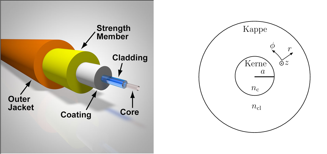
Figure 3 – Left figure shows a typical packaging of an optical fiber. On the right is a sketch of the part of the cross section where the optical field is located.
Exercise 11
Explain why we can restrict ourselves to values of \(m\) that are non-negative integers.
Exercise 12
Show that the radial part of the field, \(R(r)\), satisfies the two differential equations\[\begin{equation*} r^2 R_c''(r)+rR_c'(r)+\big(r^2\kappa^2-m^2\big)R_c(r)=0,\quad r<a,\tag{17} \end{equation*}\]\[\begin{equation*} r^2 R_{cl}''(r)+rR_{cl}'(r)-\big(r^2\sigma^2+m^2\big)R_{cl}(r)=0,\quad r>a,\tag{18} \end{equation*}\]and the boundary conditions \(R_c(a)=R_{cl}(a)\) and \(R_c'(a)=R_{cl}'(a)\), where \(\kappa=\sqrt{k^2 n_c^2-\beta^2}\) and \(\sigma=\sqrt{\beta^2-k^2 n_{cl}^2}\).
The differential equation \(x^2 y''(x)+xy'(x)+(x^2-m^2)y(x)=0\) is called Bessel’s differential equation and has the Bessel functions of the first kind, \(J_m(x)\), as solutions. The modified Bessel differential equation \(x^2 y''(x)+xy'(x)-(x^2+m^2)y(x)=0\) has Bessel functions of the second kind, \(K_m(x)\), as solutions. The Bessel functions have the property
The Bessel functions can be called in SymPy as besselj(m, x) and besselk(m, x).
Exercise 13
Show that the propagation constant \(\beta\) is determined by the equation\[\begin{equation*} \frac{uJ_{m-1}(u)}{J_m(u)} = -\frac{vK_{m-1}(v)}{K_m(v)},\tag{21} \end{equation*}\]where \(u=\kappa a\) and \(v=\sigma a\). The supported fiber modes can therefore be described by two integers: \(m\), which enters the equation, and \(\ell\), which numbers solutions to the above equation in the direction of increasing \(u\).
The supported fiber modes are called \(\mathrm{LP}_{m\ell}\) and the fundamental mode is \(\mathrm{LP}_{01}\).
Exercise 14
Make a plot of the left-hand side of (21) as a function of \(u\) and the right-hand side of (21) as a function of \(v\) for \(m=0,1,2\).
Exercise 15
Show that \(V^2=u^2+v^2\) does not depend on \(\beta\) and determine an expression for \(V\).
The parameter \(V\), which depends only on the system parameters, is called the normalized frequency.
Exercise 16
Explain why the number of solutions to equation (21) depends only on the value of \(V\).
Exercise 17
Argue (for example from the figure from Exercise 14) that, unlike the planar waveguide, the fundamental mode can, mathematically speaking, always propagate in the fiber.
Exercise 18
Determine the smallest wavelength for which only the fundamental mode can propagate in the fiber. Below this wavelength the fiber is called single-mode and almost all commercial optical fibers are designed for this regime.
In the rest of this part we consider a specific fiber with \(n_{cl}=1.444\) and \(n_c=1.450\) at wavelength \(\lambda=1.55\ \mu\mathrm{m}\), and a core radius \(a=8.0\ \mu\mathrm{m}\).
Exercise 19
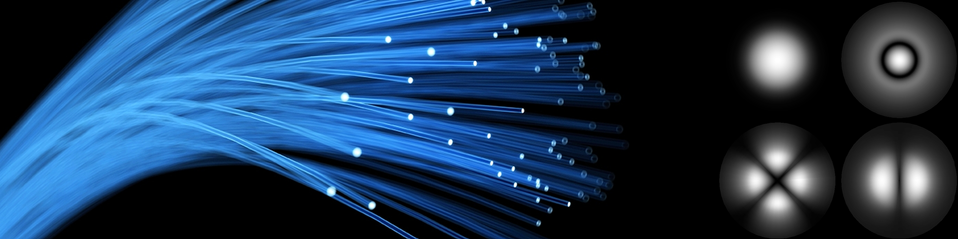
Compute the normalized frequency and state which modes can be guided in this fiber. Make heat plots of the absolute value of the transverse field distribution of these modes.
Hint: It can be an advantage to plot the two sides of (21), both as functions of \(u\). You may use Python’spcolormeshfunction from matplotlib to make heat plots (the matplotlib axes object should be created with the settingprojection='polar').
To investigate how the propagation constant depends on the light’s frequency \(\omega\), one must include that the refractive index in glass depends on frequency (or equivalently wavelength). The refractive index in the cladding, which consists of pure glass, can approximately be described by a Sellmeier equation of the form
where the parameters are given in Table 1. The refractive index in the core, which typically has been doped with a bit of germanium to increase the refractive index, can be assumed to be given by \(n_c(\omega)=n_{cl}(\omega)+\Delta n\), where the index contrast is \(\Delta n=0.006\).
Table 1 – Constants in the Sellmeier equation
\(B_1\) |
\(B_2\) |
\(B_3\) |
\(\omega_1\) (\(10^{15}\ \mathrm{s^{-1}}\)) |
\(\omega_2\) (\(10^{15}\ \mathrm{s^{-1}}\)) |
\(\omega_3\) (\(10^{15}\ \mathrm{s^{-1}}\)) |
|---|---|---|---|---|---|
0.696166300 |
0.407942600 |
0.897479400 |
27.55609797 |
16.21587137 |
0.1904734162 |
Exercise 20
Use the Sellmeier equation to plot \(n_{\mathrm{eff}}(\omega)\) from 500 nm to 2000 nm, where \(n_{\mathrm{eff}}=\beta(\omega)/k\) is the so-called effective index, which always lies between \(n_{cl}\) and \(n_c\). Do this for the four modes \(\mathrm{LP}_{01}\), \(\mathrm{LP}_{11}\), \(\mathrm{LP}_{02}\) and \(\mathrm{LP}_{21}\).
Part 3 – Quantum optics and photon-pair generation in optical fibers#
This part of the assignment is about generating pairs of photons in an optical fiber. When dealing with single photons, they behave quantum mechanically and have non-classical properties such as entanglement. The photons are generated through a nonlinear optical process called spontaneous four-wave mixing. The process is driven by an optical pump (i.e. a laser pulse) that is so weak that only a single photon pair is generated, as illustrated in Figure 4. The two photons are called signal (s) and idler (i), respectively.
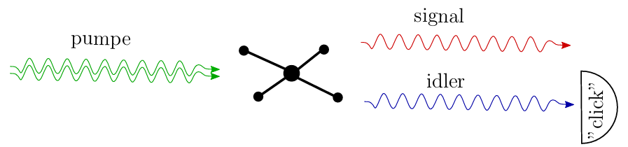
Figure 4 – Two pump photons interact nonlinearly with a glass molecule and become a signal and an idler photon, each with a frequency/wavelength that differs from the pump’s. Here the idler is detected to herald the signal photon’s presence, and the remaining signal photon can then be used.
Because signal and idler photons are quantum-mechanical particles, it is necessary to describe them with a two-particle wavefunction. One can show that the wavefunction describing the frequencies of the two photons in an optical fiber has the form
The wavefunction \(A(\Delta\omega_s,\Delta\omega_i)\) is often called the joint spectral amplitude. In (23), \(\Delta\omega_s\) denotes the deviation from a central signal frequency \(\omega_{s0}\), and similarly \(\Delta\omega_i\) denotes the idler’s deviation from a central idler frequency. \(\sigma_p\) denotes the pump’s spectral width and is given from the pump pulse’s temporal duration. As with wavefunctions in quantum mechanics, the JSA has the property that \(|A(\Delta\omega_s,\Delta\omega_i)|^2\) is a probability density for simultaneously finding the signal photon with frequency deviation \(\Delta\omega_s\) and the idler photon with frequency deviation \(\Delta\omega_i\). Furthermore, \(\beta_{1s}\), \(\beta_{1i}\) and \(\beta_{1p}\) are the first derivatives of the propagation constant with respect to \(\omega\) at the central signal, idler, and pump frequencies (e.g. \(\beta_{1s}=\beta'(\omega_{s0})\)), \(\sigma_p\) is the pump’s spectral width (measured in \(\mathrm{s^{-1}}\)), and \(L\) is the fiber length.
Exercise 21
Introduce new variables \(\nu_s=\Delta\omega_s/\sigma_p\) and \(\nu_i=\Delta\omega_i/\sigma_p\) and show that the expression can be rewritten as\[\begin{equation*} A(\nu_s,\nu_i) = \mathrm{sinc}\left(\frac{\alpha_s\nu_s+\alpha_i\nu_i}{2}\right) \exp\left[-\frac{(\nu_s+\nu_i)^2}{4}\right], \tag{24} \end{equation*}\]with appropriate definitions of the dimensionless constants \(\alpha_s\) and \(\alpha_i\).
Exercise 22
Make a 2D plot of the absolute value of \(A\) for \(\alpha_s=1\) and \(\alpha_i=0.5\).
Hint: Use for exampleimshoworpcolormeshfrom matplotlib in Python.
As an approximation, the sinc function can be replaced by a Gaussian-like function:
Exercise 23
Determine the value of \(\gamma\) such that the two functions on the left and right side of (25) have the same width when they assume half of their maximum value.
With this value of \(\gamma\) the JSA from (24) can now be approximated as:
Exercise 24
Make a 2D plot of the approximated JSA with \(\alpha_s=1\) and \(\alpha_i=0.5\) and comment on the validity of approximating the sinc function with an exponential function.
As mentioned, the absolute square of the JSA, \(|A(\nu_s,\nu_i)|^2\), is a probability density. It tells, among other things, that the probability \(dS\) of finding the signal and idler photon pair at normalized frequencies in an (vanishingly) small region around \(\nu_s\) and \(\nu_i\), respectively, is:
The constant \(N\) is a normalization constant given by
Exercise 25
Based on the approximation of the JSA in (26) with \(\alpha_s=1\) and \(\alpha_i=0.5\), compute the normalization constant \(N\). Then compute:
The probability of simultaneously detecting the signal photon at \(\nu_s\ge 0\) and the idler photon at \(\nu_i\ge 0\).
The probability of \(\nu_s\le 0\) and \(\nu_i\le 0\).
The probability for the opposite case, where \(\nu_s\ge 0\) and \(\nu_i\le 0\).
The probability of \(\nu_s\le 0\) and \(\nu_i\ge 0\).
In almost all cases the two photons in the photon pair are partially entangled, which implies a spectral correlation. That is, if one photon is detected at a particular wavelength/frequency, one obtains information about the distribution of the other photon that was not available before the measurement.
Exercise 26
Compare the results from the previous exercise with the 2D plot of the approximated JSA (with \(\alpha_s=1\) and \(\alpha_i=0.5\)). Explain why this state contains strong spectral correlations.
The correlation between the two photons can be quantified by the so-called quantum-mechanical purity of the remaining photon after the other has been detected. The quantum-mechanical purity has the maximal (and optimal) value 1 when the JSA can be factorized, i.e. written as a product of two functions that each depend on only \(\nu_s\) or \(\nu_i\): \(A(\nu_s,\nu_i)=f(\nu_s)g(\nu_i)\).
Exercise 27
Determine whether the function \(A(\nu_s,\nu_i)=(\nu_s\nu_i+3\nu_s-2\nu_i-6)\exp(-\nu_s^2-2\nu_i^2)\) can be factorized as described above.
We now investigate in which cases the state in (23) has high purity.
Exercise 28
Based on the approximation in (26), determine all values of \(\alpha_s\) and \(\alpha_i\) that make \(A(\nu_s,\nu_i)\) factorable, i.e. such that it can be written in the form \(A(\nu_s,\nu_i)=f(\nu_s)g(\nu_i)\), where \(f\) and \(g\) are two functions of one variable.
A central concept in connection with correlated quantum states is singular values. Singular values for a (non-square) matrix \(A\) are the square roots of all non-negative eigenvalues of the matrix \(AA^T\). This gives a sequence of singular values \(\lambda_1,\lambda_2,\dots\).
Exercise 29
Find, by hand calculation, all singular values for the matrix\[\begin{equation*} A= \begin{pmatrix} 3 & 2 & 2 \\ 2 & 3 & -3 \end{pmatrix}. \tag{29} \end{equation*}\]
Singular values can also be found using the numpy.linalg.svd() command in Python (remember to import NumPy). When one of the two photons is detected, the remaining single photon constitutes its own quantum-mechanical state. This state’s quantum-mechanical purity (English: purity) can be computed from the found singular values using the formula
The purity, which among other things is a measure of the degree of spectral correlation in the photon-pair state, always lies between 0 and 1, where 1 corresponds to no spectral correlation. That is, if there is no spectral correlation in the photon-pair state, then the single photon left after detecting one of the two photons will be in a so-called quantum-mechanically pure state.
Exercise 30
Compute the purity of the matrix from the previous exercise.
Exercise 31
Explain, based on expression (30), why an uncorrelated photon pair (i.e. high purity) requires that all singular values except one are zero.
Note#
In the last exercises below the complexity is increased a bit, and it is necessary to use methods from several of the earlier exercises to get through them most efficiently. It may be recommended to analyze some of the problems graphically/numerically rather than analytically, and for that it is an advantage to be comfortable using numerical methods in Python. Do not hesitate to ask for help if you get stuck.
To determine singular values for a quantum state it is necessary to represent \(A\) as a large matrix—i.e. a discretized version of the continuous 2D function. In Python, use the function lambdify((i, j), f(i, j)) from SymPy together with NumPy’s meshgrid(-N..N, -N..N) to construct a matrix with elements \(e_{ji}=f(i,j)\), where \(f(i,j)\) is a symbolic function in SymPy.
Hint: When finding singular values for a matrix, it is important to ensure that the whole state is included in the matrix.
Exercise 32
Investigate which values of the constants \(\alpha_s\) and \(\alpha_i\) give the highest purity for the JSA in (24) (without the approximation of the sinc function). What values does this require for \(\beta_{1s}-\beta_{1p}\) and \(\beta_{1i}-\beta_{1p}\) for a fiber of length \(L=10\ \mathrm{m}\) and a pump pulse that lasts 1 ps and therefore has \(\sigma_p=1\times 10^{12}\ \mathrm{s^{-1}}\)?
It is now desired to create a photon-pair state with a pump at central wavelength \(\lambda_p=1064\ \mathrm{nm}\), a signal at central wavelength \(\lambda_s=1550\ \mathrm{nm}\) and an idler at central wavelength \(\lambda_i=810\ \mathrm{nm}\). By choosing the right combination of modes for pump, signal and idler, it is possible to optimize the purity of the remaining photon when the other photon is detected.
Exercise 33
What is the highest purity you can obtain with the fiber from the end of Part 2, if the fiber length is \(L=10\ \mathrm{m}\) and the pump’s width is \(\sigma_p=1\times 10^{12}\ \mathrm{s^{-1}}\)?
Hint: Compute the first derivative of the propagation constant, \(\beta_1\), for the three fields (pump, signal and idler) in different mode combinations and use techniques from this part of the problem set to obtain a high purity.
Exercise 34
Design a fiber where the purity becomes higher than 80% for a photon-pair state with \(\lambda_p=1064\ \mathrm{nm}\), \(\lambda_s=1550\ \mathrm{nm}\) and \(\lambda_i=810\ \mathrm{nm}\). You are free to choose the length of the fiber, \(L\), the pump pulse’s temporal length, \(\sigma_p^{-1}\), the core radius \(a\), and the index contrast \(\Delta n\). Plot the resulting JSA.
Challenge: How high a purity can you achieve?