import matplotlib
if not hasattr(matplotlib.RcParams, "_get"):
    matplotlib.RcParams._get = dict.get

Linear Transformations and Matrices

Setup

We import the necessary Python packages.

import numpy as np
import matplotlib

if not hasattr(matplotlib.RcParams, "_get"):
    matplotlib.RcParams._get = dict.get

import matplotlib.pyplot as plt

Introduction

From your usual mathematics education you know functions:

\[ f(x)=x^{2}, \qquad x\in\mathbb{R}, \qquad (f:\mathbb{R}\to \mathbb{R}). \]

This means that for a value \(x\in\mathbb{R}\) we find a \(y\)-value \(f(x)\). If \(x=3\), then \(f(3)=9\).

The range of the function is

\[ \mathrm{range}(f)=[0,\infty[ . \]

which means that not all \(y\)-values can be reached by an \(x\)-value.

Think about why?

Does \(f\) have an inverse function?

We will now define a special type of functions, which take vectors, and where the value is also vectors. For example,

\[f:\mathbb{R}^{2}\to\mathbb{R}^{2}.\]

Before we define these new functions, we must introduce a new concept called matrices.

Matrices

Examples

A real \(2\times 2\) matrix is a scheme with numbers:

\[\begin{split} M_1 = \begin{bmatrix} 1 & 2 \\ 3 & 4 \end{bmatrix} \qquad \text{is a $2\times 2$ matrix.} \end{split}\]

Another example:

\[\begin{split} M_{2}=\begin{bmatrix}1 & 2 & 3 \\ 4 & 5 & 6\end{bmatrix}\qquad\text{is a }2\times 3\text{ matrix.} \end{split}\]

We talk about columns and rows in matrices.

\(M_{2}\) has 2 rows:

\[ \begin{bmatrix} 1 & 2 & 3 \end{bmatrix} \quad \text{is row 1,} \qquad \begin{bmatrix} 4 & 5 & 6 \end{bmatrix} \quad \text{is row 2.} \]

\(M_{2}\) has 3 columns:

\[\begin{split} \begin{bmatrix} 1 \\ 4 \end{bmatrix} \quad \text{is column 1,} \qquad \begin{bmatrix} 2 \\ 5 \end{bmatrix} \quad \text{is column 2,} \qquad \begin{bmatrix} 3 \\ 6 \end{bmatrix} \quad \text{is column 3.} \end{split}\]

Matrix-vector product

We now introduce a matrix-vector product.

\[\begin{split} M = \begin{bmatrix} \text{---} & \boldsymbol{r}_1 & \text{---} \\ \text{---} & \boldsymbol{r}_2 & \text{---} \\ &\vdots \\ \text{---} & \boldsymbol{r}_m & \text{---} \end{bmatrix}_{m \text{ rows}, \; n \text{ columns}} \qquad \boldsymbol{v} = \begin{bmatrix} v_{1} \\ v_{2} \\ \vdots \\ v_{n} \end{bmatrix}_{n \text{ rows}, \; 1 \text{ column}}. \end{split}\]

Here, \(\;\boldsymbol{r}_1,\dots,\boldsymbol{r}_m\;\) are the \(m\) rows in \(M\).

\[\begin{split} M\boldsymbol{v} = \begin{bmatrix} \boldsymbol{r}_1 \cdot \boldsymbol{v} \\ \boldsymbol{r}_2 \cdot \boldsymbol{v} \\ \vdots \\ \boldsymbol{r}_m \cdot \boldsymbol{v} \end{bmatrix}. \end{split}\]

where each row consists of the usual dot product between the corresponding row in \(M\) and the vector \(\boldsymbol{v}\).

Note: The number of columns in \(M\) must match the number of rows in \(\boldsymbol{v}\).

Consider for example the matrix and vector

\[\begin{split} M=\begin{bmatrix}1 & 2 \\ 3 & 4\end{bmatrix}, \qquad \boldsymbol{v}=\begin{bmatrix}-1 \\ 1\end{bmatrix}. \end{split}\]

We can calculate the product as

\[\begin{split} M \boldsymbol{v} = \begin{bmatrix} 1 & 2 \\ 3 & 4 \end{bmatrix} \begin{bmatrix} -1 \\ 1 \end{bmatrix} = \begin{bmatrix} 1\cdot(-1)+2\cdot 1 \\ 3\cdot(-1)+4\cdot 1 \end{bmatrix} = \begin{bmatrix} 1 \\ 1 \end{bmatrix}. \end{split}\]

In Python, it is calculated as follows.

M = np.array([[1,2],[3,4]])
v = np.array([-1,1])
print(M @ v)

[1 1]

Let’s try. Consider the four following matrix-vector pairs:

\[\begin{split} M_{1} = \begin{bmatrix} -1 & 0 \\ 0 & 1 \end{bmatrix}, \quad \boldsymbol{v}_{1} = \begin{bmatrix} 2 \\ 3 \end{bmatrix}. \end{split}\]

\[\begin{split} M_{2} = \begin{bmatrix} 1 & 0 & 2 \\ 0 & -2 & 3 \end{bmatrix}, \quad \boldsymbol{v}_{2} = \begin{bmatrix} 2 \\ 3 \end{bmatrix}. \end{split}\]

\[\begin{split} M_{3} = \begin{bmatrix} 1 & 0 & 2 \\ 0 & -2 & 3 \end{bmatrix}, \quad \boldsymbol{v}_{3} = \begin{bmatrix} -1 \\ -2 \\ 3 \end{bmatrix}. \end{split}\]

\[\begin{split} M_{4} = \begin{bmatrix} 1 & 2 \\ 3 & 0 \\ -1 & 4 \end{bmatrix}, \quad \boldsymbol{v}_{4} = \begin{bmatrix} 2 \\ 3 \end{bmatrix}. \end{split}\]

Try to perform each matrix-vector product by hand, and determine which of the 4 cannot be performed.

Use the following code cell to see if you get the same result in Python.

# Calculate matrix-vector products here

Can you make a rule for the number of rows and columns in the product \(M\boldsymbol{v}\) based on knowledge of the number of columns and rows in \(M\) and \(v\) respectively?

Back to Functions

We now return to functions. Let \(A\) be a \(2\times 2\) matrix.

Linear Mapping

An example of a linear mapping is

\[ f : \mathbb{R}^2 \to \mathbb{R}^2, \qquad f(\boldsymbol{v}) = A \boldsymbol{v}. \]

We can see that it always works out: Any vector \(\boldsymbol{v}\in\mathbb{R}^2\) can be multiplied by a \(2\times 2\) matrix.

The question is now: Which values can the function take?
(They lie of course in \(\mathbb{R}^2\).)

We already know that the vector

\[\begin{split} \begin{bmatrix} 0 \\ 0 \end{bmatrix} \end{split}\]

always lies in the range (which is called the image).

Why?

Note that we can write

\[\begin{split} f(\mathbf{v}) = \begin{bmatrix} | & | \\ s_1 & s_2 \\ | & | \end{bmatrix} \begin{bmatrix} v_{1} \\ v_{2} \end{bmatrix} = \begin{bmatrix} | \\ s_{1} \\ | \end{bmatrix} v_{1} + \begin{bmatrix} | \\ s_{2} \\ | \end{bmatrix} v_{2}, \end{split}\]

where \(s_1\) and \(s_2\) are the columns in \(A\).

Can you explain why this holds?

This figure is created in the following code cell.

# --- input (experiment with the numerical values here) ---
s1 = np.array([1, 3])   # first column
s2 = np.array([2, 0.5])   # second column
v1, v2 = 2, 3           # elements in the vector
# ------------------------------------------

f_v = v1*s1 + v2*s2

fig, ax = plt.subplots()

# draw column products
ax.quiver(0, 0, *v1*s1, angles='xy', scale_units='xy', scale=1, color="blue")
ax.text(*v1*s1/2, r'$v_1\mathbf{s}_1$', fontsize=12, color="k", ha='left', va='top')
ax.plot([v1*s1[0], f_v[0]], [v1*s1[1], f_v[1]], 'b--', linewidth=1)
ax.quiver(0, 0, *v2*s2, angles='xy', scale_units='xy', scale=1, color="blue")
ax.text(*v2*s2/2, r'$v_2\mathbf{s}_2$', fontsize=12, color="k", ha='left', va='top')
ax.plot([v2*s2[0], f_v[0]], [v2*s2[1], f_v[1]], 'b--', linewidth=1)

# draw columns
ax.quiver(0, 0, *s1, angles='xy', scale_units='xy', scale=1, color="green")
ax.text(*s1/2, r'$\mathbf{s}_1$', fontsize=12, color="k", ha='right', va='bottom')
ax.quiver(0, 0, *s2, angles='xy', scale_units='xy', scale=1, color="green")
ax.text(*s2/2, r'$\mathbf{s}_2$', fontsize=12, color="k", ha='right', va='bottom')

# draw f(v)
ax.quiver(0, 0, *f_v, angles='xy', scale_units='xy', scale=1, color="r")
ax.text(*f_v/2, r'$f(\mathbf{v})$', fontsize=12, color="k", ha='right', va='bottom')

# plot appearance
ax.axhline(0, color="black", linewidth=1)
ax.axvline(0, color="black", linewidth=1)
ax.set_aspect("equal")
ax.set_xlim(min(v1*s1[0], v2*s2[0], f_v[0], 0) - 1, max(v1*s1[0], v2*s2[0], f_v[0], 0) + 1)
ax.set_ylim(min(v1*s1[1], v2*s2[1], f_v[1], 0) - 1, max(v1*s1[1], v2*s2[1], f_v[1], 0) + 1)
ax.grid(True, which='both', linestyle='--', linewidth=0.5)
ax.set_xlabel("$x$")
ax.set_ylabel("$y$")

plt.show()

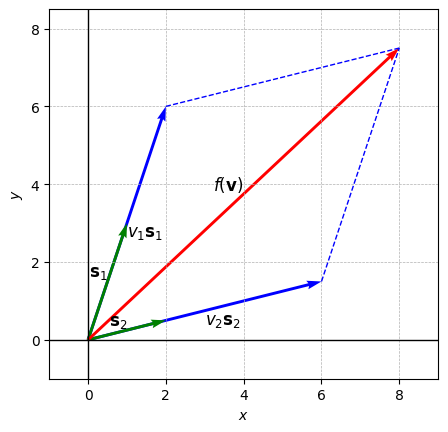
Explain from the figure why the range is either the point \((0,0)\), a straight line through the origin, or the entire \(\mathbb{R}^2\).
Hint: What happens if the two columns are parallel? Try it by changing the numerical values for the figure.

Exercise

Let

\[\begin{split} A = \begin{bmatrix}0 & 0 \\ 0 & 0\end{bmatrix}, \quad B = \begin{bmatrix}1 & 1 \\ -1 & 1\end{bmatrix}, \quad C = \begin{bmatrix}1 & -2 \\ -1 & 2\end{bmatrix} \end{split}\]

and

\[\begin{split} \boldsymbol{v}_{1} = \begin{bmatrix}1 \\ 1\end{bmatrix}, \quad \boldsymbol{v}_{2} = \begin{bmatrix}-1 \\ 1\end{bmatrix}. \end{split}\]

Define the functions \(f_A(\boldsymbol{v})=A\boldsymbol{v}\), \(f_B(\boldsymbol{v})=B\boldsymbol{v}\), \(f_C(\boldsymbol{v})=C \boldsymbol{v}\).

Set up in the following code cell the matrices \(A,\;B\) and \(C\) as well as the vectors \(\boldsymbol{v}_1\) and \(\boldsymbol{v}_2\).

#

Calculate \(f_{A}(v_{1})\), \(f_{A}(v_{2})\), \(f_{B}(v_{1})\), \(f_{B}(v_{2})\), \(f_{C}(v_{1})\) and \(f_{C}(v_{2})\) and inspect the results using print.

print(s1)

[1 3]

Let’s try to visualize it. In the following code cell, the draw_vectors function is defined, which we can use to show vectors in a coordinate system.

def draw_vectors(vector_list):
    # input: list of 2D vectors as numpy arrays

    fig, ax = plt.subplots()
    
    # draw the vectors
    for v in vector_list:
        ax.quiver(0, 0, *v, angles='xy', scale_units='xy', scale=1, color="blue")
        #ax.text(*(v/2), f"({v[0]}, {v[1]})",fontsize=10, color="k", ha='right', va='bottom')
    
    # set the plot size
    all_x = [v[0] for v in vector_list] + [0]
    all_y = [v[1] for v in vector_list] + [0]
    ax.set_xlim(min(all_x) - 1, max(all_x) + 1)
    ax.set_ylim(min(all_y) - 1, max(all_y) + 1)

    # plot appearance
    ax.axhline(0, color="black", linewidth=1)
    ax.axvline(0, color="black", linewidth=1)
    ax.set_aspect("equal")
    ax.grid(True, which='both', linestyle='--', linewidth=0.5)
    ax.set_xlabel("$x$")
    ax.set_ylabel("$y$")

    plt.show()

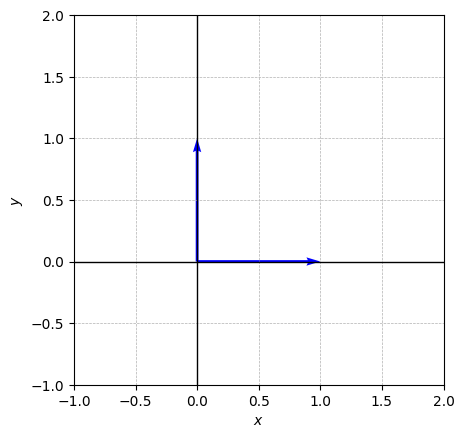
Use the function to visualize the image vectors within the same coordinate system.

vector_list = [np.array([1,0]), np.array([0,1])]
draw_vectors(vector_list)

Try to describe the range of the three functions. Think about which vectors in \(\mathbb{R}^2\) can be reached by \(f_A\), \(f_B\) and \(f_C\) when \(\boldsymbol{v} \in \mathbb{R}^2\)?

Rank

We will introduce the concept of rank of a matrix.

Ask your favorite AI about the concept of rank.

In Python, the rank of a matrix can be calculated with the function np.linalg.matrix_rank(M).

Determine \(\;\text{rank}(A),\;\text{rank}(B)\) and \(\text{rank}(C)\).

#

Note: It is only for the function \(f_B\) that we can find an inverse function.

Why?

Rotations

We now consider a special class of functions:

\[\begin{split} f(\boldsymbol{v})=M\boldsymbol{v},\qquad M = \begin{bmatrix}\cos\theta & -\sin\theta \\ \sin\theta & \cos\theta\end{bmatrix}, \qquad -\pi \le \theta \le \pi. \end{split}\]

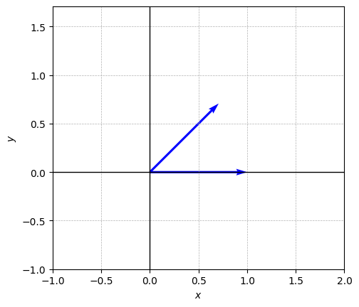
\(M\) thus rotates a vector \(\boldsymbol{v}\) by \(\theta\) radians in the positive direction. In the following code cell we rotate the vector \(\boldsymbol{e}_1=\begin{bmatrix} 1\\0\end{bmatrix}\) by \(\frac{\pi}{4}\) radians (\(45^{\circ}\)).

e1 = np.array([1,0])
theta = np.pi/4
M = np.array([[np.cos(theta), -np.sin(theta)],
              [np.sin(theta),  np.cos(theta)]])
draw_vectors([e1, M @ e1])

Exercise

Of the following 5 matrices, some correspond to a rotation as above.

\[\begin{split} M_{1}=\begin{bmatrix}0 & -1 \\ 1 & 0\end{bmatrix}, \quad M_{2}=\begin{bmatrix}1 & 0 \\ 0 & 1\end{bmatrix}, \quad M_{3}=\begin{bmatrix}\tfrac{1}{\sqrt{2}} & -\tfrac{1}{\sqrt{2}} \\ \tfrac{1}{\sqrt{2}} & \tfrac{1}{\sqrt{2}}\end{bmatrix}, \end{split}\]

\[\begin{split} M_{4}=\begin{bmatrix}1 & -1 \\ 1 & 1\end{bmatrix}, \quad M_{5}=\begin{bmatrix}\tfrac{1}{2} & \tfrac{\sqrt{3}}{2} \\ -\tfrac{\sqrt{3}}{2} & \tfrac{1}{2}\end{bmatrix}. \end{split}\]

Which of the following 5 matrices correspond to a rotation as above.

For each of the matrices, try to draw a vector \(\boldsymbol{v}\) and the image vector \(f(\boldsymbol{v})\) in the same coordinate system (you can use draw_vectors as above).
Does the angle appear to match?

#

We can advantageously define a Python function that returns a rotation matrix for a given angle \(\theta\).

Complete the function rotation_matrix in the following code cell.

def rotation_matrix(theta):
    """
    Returns a 2D rotation matrix for a rotation by angle theta (in radians).
    """
    # OWN CODE: Define the rotation matrix M
    M =

    return M

  Cell In[12], line 6
    M =
       ^
SyntaxError: invalid syntax

With this function we can now define a rotation matrix \(M\) as M=rotation_matrix(theta).

Test your function by recreating one of the five matrices above using the angle you found. Hint: In Python, \(\pi\) is obtained by np.pi.

#

Explanation: why \(f\) corresponds to a rotation

A vector \(v\) can be understood as a length and a direction, we can write

\[\begin{split} \boldsymbol{v} = |\boldsymbol{v}|\begin{bmatrix} \cos\alpha \\ \sin\alpha \end{bmatrix}, \end{split}\]

where \(\alpha\) corresponds to the angle between the vector and the \(x\)-axis (the positive direction).

Now try to perform the matrix-vector product:

\[\begin{split} M \boldsymbol{v} = |\boldsymbol{v}|\begin{bmatrix} \cos\theta & -\sin\theta \\ \sin\theta & \cos\theta \end{bmatrix} \begin{bmatrix} \cos\alpha \\ \sin\alpha \end{bmatrix}. \end{split}\]

Try to ask your favorite AI what addition formulas are,
and see if you can answer the question using these:
Why does \(f\) correspond to a rotation of \(\theta\) radians in the positive direction?

How can it be that \(|\boldsymbol{v}|\) could be moved outside the matrix product?

Matrix-matrix product

We define a matrix-matrix product analogously with the matrix-vector product.

Let

\[\begin{split} M= \left[ \begin{array}{cccc} m_{11} & m_{12} & \cdots & m_{1n}\\ m_{21} & m_{22} & \cdots & m_{2n}\\ \vdots & \vdots & \ddots & \vdots\\ m_{m1} & m_{m2} & \cdots & m_{mn} \end{array} \right] \qquad \begin{array}{l} \text{$n$ columns}\\ \text{$m$ rows} \end{array} \end{split}\]

and

\[\begin{split} N= \left[ \begin{array}{cccc} n_{11} & n_{12} & \cdots & n_{1k}\\ \vdots & \vdots & \ddots & \vdots\\ n_{n1} & n_{n2} & \cdots & n_{nk} \end{array} \right] \qquad \begin{array}{l} \text{$k$ columns}\\ \text{$n$ rows} \end{array} \end{split}\]

Then

\[\begin{split} M\,N = \left[ \begin{array}{cccc} \alpha_{11} & \alpha_{12} & \cdots & \alpha_{1k}\\ \alpha_{21} & \alpha_{22} & \cdots & \alpha_{2k}\\ \vdots & \vdots & \ddots & \vdots\\ \alpha_{m1} & \alpha_{m2} & \cdots & \alpha_{mk} \end{array} \right], \end{split}\]

where \(\alpha_{ij}\) equals the scalar product between row \(i\) in \(M\) and column \(j\) in \(N\).

Do we get the same result with the matrix-matrix product as with the matrix-vector product in the special case where \(N\) has only one column (\(k=1\))?

Example

Consider the matrix-matrix product

\[\begin{split} \begin{bmatrix} 1 & 2\\ 3 & 4 \end{bmatrix} \begin{bmatrix} 1 & 0 & 2\\ -1 & 3 & 1 \end{bmatrix} = \begin{bmatrix} -1 & 6 & 4\\ -1 & 12 & 10 \end{bmatrix}. \end{split}\]

Can you get the same values in the product matrix as in the example?

In Python, the matrix-matrix product is performed in the same way as the matrix-vector product using @.

Verify the result above in the following code cell.

#

Back to Rotations

Exercise

Use the code cell below to answer the exercise. Specify a \(2\times2\) matrix \(M_{1}\) that rotates a vector in the positive direction by \(\tfrac{\pi}{4}\) radians, and another \(M_{2}\) that rotates a vector in the negative direction by \(\tfrac{\pi}{2}\) radians:

Now choose a vector \(v\in\mathbb{R}^{2}\).

1. First rotate the vector using \(M_1\):

\[ \boldsymbol{v}_1 = M_1 \boldsymbol{v}. \]

2. Then rotate \(v_1\) using \(M_2\):

\[ \boldsymbol{v}_2 = M_2 \boldsymbol{v}_1. \]

3. (Compare) Also calculate

\[ \boldsymbol{v}_2' = (M_2 M_1) \boldsymbol{v} \]

and compare \(\boldsymbol{v}_2'\) with \(\boldsymbol{v}_2\) (e.g., in a plot or using print).

4. Try to formulate in words what you see!

M1 = 
M2 = 
v =

  Cell In[15], line 1
    M1 =
         ^
SyntaxError: invalid syntax

Composition of rotations explanation

Let

\[\begin{split} M_{1}= \begin{bmatrix} \cos\theta_{1} & -\sin\theta_{1}\\ \sin\theta_{1} & \ \cos\theta_{1} \end{bmatrix} \qquad\text{and}\qquad M_{2}= \begin{bmatrix} \cos\theta_{2} & -\sin\theta_{2}\\ \sin\theta_{2} & \ \cos\theta_{2} \end{bmatrix}. \end{split}\]

be two rotation matrices.

Calculate \(M_{1}M_{2}\) by hand.

Now use the addition formulas from earlier to show that \(M_{1}M_{2}\) has the same effect as a rotation by angle \(\theta_{1}+\theta_{2}\) on any vector in \(\mathbb{R}^{2}\).

Example: Reflection

Consider the matrix

\[\begin{split} M = \begin{bmatrix} 0 & 1 \\ 1 & 0 \end{bmatrix} \end{split}\]

and let \(f\) be the function \(f(\boldsymbol{v}) = M \boldsymbol{v}\).

Try with different vectors \(\boldsymbol{v}\) to find the image vector \(f(\boldsymbol{v})\).
What effect does the matrix \(M\) have on a vector?

Note that the effect of \(M\) does not correspond to a rotation in the positive direction as described above, that is, \(M\) cannot be brought into the form

\[\begin{split} \begin{bmatrix} \cos\theta & -\sin\theta \\ \sin\theta & \cos\theta \end{bmatrix}. \end{split}\]

Why not?

The effect of \(M\) on the vector \(\boldsymbol{v}\) is called a reflection, (in this case a reflection in the line spanned by the vector \(\boldsymbol{w} = (1,1)\) ).

Inverse matrix

We again consider a rotation, given by

\[\begin{split} M = \begin{bmatrix} \cos\theta & -\sin\theta \\ \sin\theta & \cos\theta \end{bmatrix}. \end{split}\]

\(M\) thus rotates \(\boldsymbol{v}\) by \(\theta\) radians in the positive direction.

Now consider the rotation matrix that rotates a vector \(\boldsymbol{v}\) by \(\theta\) radians in the negative direction:

\[\begin{split} M^{-1} = \begin{bmatrix} \cos(-\theta) & -\sin(-\theta) \\ \sin(-\theta) & \cos(-\theta) \end{bmatrix} = \begin{bmatrix} \cos\theta & \sin\theta \\ -\sin\theta & \cos\theta \end{bmatrix}. \end{split}\]

Explain why the two matrices mentioned above look the way they do.

It is clear from the definition of \(M\) and \(M^{-1}\) that

\[ M^{-1}(M\boldsymbol{v}) = M(M^{-1}\boldsymbol{v}) = \boldsymbol{v}. \]

Try with different angles and vectors to verify the above identities.

Now try with the same angles to calculate the matrix-matrix products \(M^{-1}M\) and \(MM^{-1}\).
What do you see?

We call

\[\begin{split} \begin{bmatrix} 1 & 0 \\ 0 & 1 \end{bmatrix} \end{split}\]

the identity matrix \(I\).

What effect does it have on a vector?

We say that a matrix \(M\) with equal number of columns and rows has an inverse matrix if there exists a matrix \(M^{-1}\) with the property

\[ M^{-1}M = MM^{-1} = I. \]

Diagonal matrix

A matrix of the form

\[\begin{split} D = \begin{bmatrix} m_{11} & 0 & 0 & \cdots & 0 \\ 0 & m_{22} & 0 & \cdots & 0 \\ 0 & 0 & \ddots & \ddots & 0 \\ \vdots & \vdots & \ddots & \ddots & \vdots \\ 0 & 0 & 0 & \cdots & m_{nn} \end{bmatrix}, \end{split}\]

where only the diagonal elements are nonzero (note that we call the diagonal the line that goes from the upper left corner to the lower right corner in the matrix).

The identity matrix is a diagonal matrix – why?

Consider the four following examples of \(2\times 2\) diagonal matrices:

\[\begin{split} D_{1} = \begin{bmatrix} -1 & 0 \\ 0 & 1 \end{bmatrix}, \quad D_{2} = \begin{bmatrix} 2 & 0 \\ 0 & 3 \end{bmatrix}, \quad D_{3} = \begin{bmatrix} \frac{1}{2} & 0 \\ 0 & \frac{1}{3} \end{bmatrix}, \quad D_{4} = \begin{bmatrix} 0 & 0 \\ 0 & 2 \end{bmatrix}. \end{split}\]

Try to find the inverse matrix (if possible) for the four diagonal matrices.

The matrix

\[\begin{split} V = \begin{bmatrix} 0 & -1 \\ \frac{1}{2} & 0 \end{bmatrix} \end{split}\]

is not a diagonal matrix.

Why not?

Can you find an inverse of \(V\)?

To see the effect of a diagonal matrix on a vector \(\boldsymbol{v}\), we now consider the function again

\[ f(\boldsymbol{v}) = N_i \boldsymbol{v}, \]

where

\[\begin{split} N_{1} = \begin{bmatrix} 1 & 0 \\ 0 & 1 \end{bmatrix}, \quad N_{2} = \begin{bmatrix} 2 & 0 \\ 0 & 2 \end{bmatrix}, \quad N_{3} = \begin{bmatrix} 1 & 0 \\ 0 & 2 \end{bmatrix}, \quad N_{4} = \begin{bmatrix} 0 & 1 \\ -1 & 0 \end{bmatrix}. \end{split}\]

Calculate \(f(\boldsymbol{v})\) in these 4 cases, use different \(\boldsymbol{v}\)’s.

#

Can you explain the effect on a vector \(\boldsymbol{v}\) in the 4 cases?

Composition of rotations and diagonal matrices

We again consider the 4 matrices above. Let \(M\) be the matrix

\[\begin{split} M = \begin{bmatrix} \cos\left(\tfrac{\pi}{4}\right) & -\sin\left(\tfrac{\pi}{4}\right) \\ \sin\left(\tfrac{\pi}{4}\right) & \cos\left(\tfrac{\pi}{4}\right) \end{bmatrix}. \end{split}\]

Now calculate \(M^{-1}N_iM\) and explain the result using a plot.

#

Do the same rules apply as for numbers, that the order of the factors is irrelevant, that is, is it correct that:

\[ M^{-1}N_iM = N_iM^{-1}M = N_i I = N_i \, ? \]

If it does not apply generally, is it always wrong?

Rotation of coordinate system and change of coordinates

We now consider two coordinate systems, our usual \(x\)-\(y\) coordinate system and then a new rotated \(x'\)-\(y'\) coordinate system. The figure is generated by running the following code cell.

# Rotation angle
theta = np.pi / 6

# Axis definitions
x_axis = np.array([1, 0])
y_axis = np.array([0, 1])
x_prime = np.array([np.cos(theta), np.sin(theta)])
y_prime = np.array([-np.sin(theta), np.cos(theta)])

# The vector v
v = np.array([np.cos(np.pi/4), np.sin(np.pi/4)])

fig, ax = plt.subplots(figsize=(5, 5))

# Plot the axes
axes_width = 0.004
ax.quiver(0, 0, *x_axis, angles="xy", scale_units="xy", scale=1, color="black", width=axes_width)
ax.text(1.05, -0.05, "$x$", fontsize=12)

ax.quiver(0, 0, *y_axis, angles="xy", scale_units="xy", scale=1, color="black", width=axes_width)
ax.text(-0.05, 1.05, "$y$", fontsize=12)

ax.quiver(0, 0, *x_prime, angles="xy", scale_units="xy", scale=1, color="black", width=axes_width)
ax.text(x_prime[0]+0.05, x_prime[1], "$x'$", fontsize=12)

ax.quiver(0, 0, *y_prime, angles="xy", scale_units="xy", scale=1, color="black", width=axes_width)
ax.text(y_prime[0]-0.1, y_prime[1], "$y'$", fontsize=12)

# Plot the vector v
ax.quiver(0, 0, *v, angles="xy", scale_units="xy", scale=1, color="black", width=0.006)
ax.text(v[0]+0.05, v[1]+0.05, r"the vector $\mathbf{v}$", fontsize=12)

# Angle arc for theta
arc = np.linspace(0, theta, 100)
ax.plot(0.4*np.cos(arc), 0.4*np.sin(arc), color="black",linewidth=1)
ax.text(0.5*np.cos(theta/2), 0.5*np.sin(theta/2), r"$\theta$", fontsize=12)

# Plot appearance
ax.set_aspect('equal')
ax.set_xlim(-1, 1.5)
ax.set_ylim(-0.5, 1.5)
ax.axis("off")

plt.show()

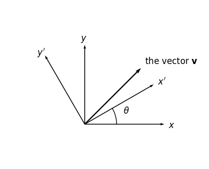
The task is now, if we know the coordinates of \(\boldsymbol{v}\) in the usual coordinate system, to find the coordinates in the rotated coordinate system and vice versa.

---

First an easy example: Let us rotate the \(x'\)-\(y'\)-coordinate system \(\tfrac{\pi}{2}\) radians with respect to the \(x\)-\(y\)-coordinate system.

# Rotation angle
theta = np.pi / 2

# Axis definitions
x_axis = np.array([2, 0])
y_axis = np.array([0, 2])
x_prime = 2*np.array([np.cos(theta), np.sin(theta)])
y_prime = 2*np.array([-np.sin(theta), np.cos(theta)])

# The vector v
v = np.sqrt(2)*np.array([np.cos(np.pi/4), np.sin(np.pi/4)])

fig, ax = plt.subplots(figsize=(5, 5))

# Plot the axes
axes_width = 0.004
ax.quiver(0, 0, *x_axis, angles="xy", scale_units="xy", scale=1, color="black", width=axes_width)
ax.text(x_axis[0]+0.05, x_axis[1], "$x$", fontsize=12)

ax.quiver(0, 0, *y_axis, angles="xy", scale_units="xy", scale=1, color="black", width=axes_width)
ax.text(y_axis[0]-0.1, y_axis[1], "$y$", fontsize=12)

ax.quiver(0, 0, *x_prime, angles="xy", scale_units="xy", scale=1, color="black", width=axes_width)
ax.text(x_prime[0]+0.05, x_prime[1], "$x'$", fontsize=12)

ax.quiver(0, 0, *y_prime, angles="xy", scale_units="xy", scale=1, color="black", width=axes_width)
ax.text(y_prime[0]-0.1, y_prime[1], "$y'$", fontsize=12)

# Plot the vector v and projections on the x and y axes
ax.quiver(0, 0, *v, angles="xy", scale_units="xy", scale=1, color="black", width=0.006)
ax.text(v[0]+0.05, v[1]+0.05, r"$\mathbf{v}$", fontsize=12)
ax.plot([v[0], v[0]], [-0.05, v[1]], 'k--', linewidth=0.5)  # vertical from x-axis to tip
ax.plot([-0.05, v[0]], [v[1], v[1]], 'k--', linewidth=0.5)  # horizontal from y-axis to tip
ax.text(v[0], -0.1, "1", fontsize=10, ha='center', va='top')
ax.text(-0.1, v[1], "1", fontsize=10, ha='right', va='center')

# Plot appearance
ax.axis('off')
ax.set_aspect('equal')
ax.set_xlim(-2.5, 2.5)
ax.set_ylim(-1, 3)

plt.show()

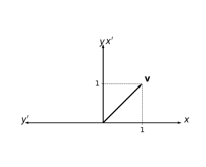
The coordinates of \(\boldsymbol{v}\) with respect to the \(x\)-\(y\)-coordinate system are

\[ (1,1). \]

The coordinates of \(\boldsymbol{v}\) with respect to the \(x'\)-\(y'\)-coordinate system are

\[ (1,-1). \]

Explain why, use the figure.

---

Now we return to the original problem.

Let us say that the coordinates of \(\boldsymbol{v}\) with respect to the \(x'\)-\(y'\)-coordinate system are

\[ (v_1',v_2'), \]

Imagine now that the two coordinate systems are coinciding at the start, and then we start rotating the \(x'\)-\(y'\)-coordinate system by \(\theta\) radians in the positive direction with the vector \(\boldsymbol{v}\) attached to the \(x'\)-\(y'\)-coordinate system.

This corresponds to rotating the vector \(\boldsymbol{v}\) by \(\theta\) radians, so the coordinates in the \(x\)-\(y\)-coordinate system are

\[\begin{split} \begin{pmatrix} x \\[0.3em] y \end{pmatrix} = \begin{bmatrix} \cos\theta & -\sin\theta \\ \sin\theta & \cos\theta \end{bmatrix} \begin{pmatrix} x' \\[0.3em] y' \end{pmatrix}. \end{split}\]

The rotation the opposite way is given by

\[\begin{split} \begin{pmatrix} x'\\[0.2em] y' \end{pmatrix} = \begin{bmatrix} \cos\theta & \sin\theta\\ -\sin\theta & \cos\theta \end{bmatrix} \begin{pmatrix} x\\[0.2em] y \end{pmatrix}. \end{split}\]

Explain why!

We call the two matrices involved change of coordinate matrices.

---

Exercise

Now choose a rotation angle of \(\tfrac{\pi}{4}\) radians.

1. Consider a vector \(\boldsymbol{v}\) with coordinates

\[\begin{split} \begin{pmatrix} x \\ y \end{pmatrix} = \begin{pmatrix} 1 \\ 2 \end{pmatrix}. \end{split}\]

Find the \(x'\)-\(y'\)-coordinates.

#

2. Consider a vector \(\boldsymbol{w}'\) with coordinates

\[\begin{split} \begin{pmatrix} x' \\ y' \end{pmatrix} = \begin{pmatrix} \sqrt{2} \\ \sqrt{2} \end{pmatrix}. \end{split}\]

Find the \(x\)-\(y\)-coordinates.

#

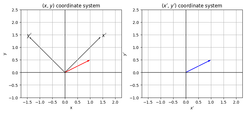
3. Let’s try to visualize this rotation. In the following code cell, two coordinate systems are generated, one each in \((x,y)\) and \((x',y')\) coordinates. In each coordinate system, an example of a vector is also plotted with the code line:

ax.quiver(0, 0, *np.array([1,1/2]), angles="xy", scale_units="xy", scale=1, color="red", width=0.006)

Make changes to the plot so we get the following:

• In the (\(x,y\))-coordinate system vectors \(\boldsymbol{v}\) and \(\boldsymbol{w}\) are shown.

• In the (\(x',y'\))-coordinate system vectors \(\boldsymbol{v}'\) and \(\boldsymbol{w}'\) are shown.

• \(\boldsymbol{v}\) and \(\boldsymbol{v}'\) are plotted with the same color, while \(\boldsymbol{w}\) and \(\boldsymbol{w}'\) have another common color.

# Rotation angle
theta = np.pi / 4

# Axis definitions
x_prime = 2*np.array([np.cos(theta), np.sin(theta)])
y_prime = 2*np.array([-np.sin(theta), np.cos(theta)])

fig, axs = plt.subplots( 1, 2, figsize = (10,10)) # create two plots side by side (1x2)

# common plot appearance
for ax in axs:
    ax.grid()
    ax.set_aspect('equal')
    ax.set_xlim(-1.75, 2.25)
    ax.set_ylim(-1, 2.5)
    ax.axhline(0, color="black", linewidth=1)
    ax.axvline(0, color="black", linewidth=1)

# left subplot (x-y coordinate system) ----------------------------
ax = axs[0]

# set axis labels and title
ax.set_xlabel('x')
ax.set_ylabel('y')
ax.set_title('($x$, $y$) coordinate system')

# plot x'-y' axes
ax.quiver(0, 0, *x_prime, angles="xy", scale_units="xy", scale=1, color="black", width=0.004)
ax.text(x_prime[0]+0.05, x_prime[1], "$x'$", fontsize=12)
ax.quiver(0, 0, *y_prime, angles="xy", scale_units="xy", scale=1, color="black", width=0.004)
ax.text(y_prime[0]-0.1, y_prime[1], "$y'$", fontsize=12)

# OWN CODE: plot vectors v and w (x-y coordinates)
ax.quiver(0, 0, *np.array([1,1/2]), angles="xy", scale_units="xy", scale=1, color="red", width=0.006) # example (remove this)

# right subplot (x'-y' coordinate system) ----------------------------
ax = axs[1]

# set axis labels and title
ax.set_xlabel("$x'$")
ax.set_ylabel("$y'$")
ax.set_title("($x'$, $y'$) coordinate system")

# OWN CODE: plot vectors v' and w' (x'-y' coordinates)
ax.quiver(0, 0, *np.array([1,1/2]), angles="xy", scale_units="xy", scale=1, color="blue", width=0.006) # example (remove this)

plt.show()