Waste Landfills: Leaching & Groundwater Transport

About the project

• Duration: 20–50 hours (including typesetting final report in LaTeX)

• Prerequisites: Differential equations (1st/2nd order), basic linear algebra (systems, eigenvalues/diagonalization), basic calculus (derivatives/integration), basic Python programming

• Python packages: NumPy, matplotlib, sympy, scipy

• Learning objectives: Model groundwater flow with Darcy’s law, set up and analyze (non)linear ODE models for hydraulic head, solve boundary value problems via matrix methods/diagonalization, fit model parameters to data via error minimization, estimate contaminant travel time from velocity and integration

Introduction

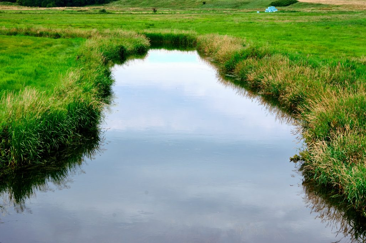
Pollution is a global—and a local—problem. Pollution from the surrounding soil areas is transported to streams, among other things via groundwater flow. This pollution can, for example, consist of pesticides that are sprayed on fields or, in rarer cases, of non-recyclable waste that is placed in so-called landfills. The pollution can pose a threat to the plants and animals that live in the water.

The purpose of the assignment is to analyze a simple model of how pollution is transported by groundwater flow. Physically, such transport is described by Darcy’s law for fluid flows:

\[ Q=-K\cdot A\frac{\partial h}{\partial x} \]

Darcy’s law corresponds to Ohm’s law for electrical circuits, where \(K\) corresponds to the conductance (1/resistance) and \(A\) is a cross-sectional area. The pressure gradient \(\partial h/\partial x\) drives the flow.

Mathematically, the project concerns topics such as solving linear and nonlinear differential equations for the pressure, \(h(x)\), via numerical and exact methods (e.g. via diagonalization). In addition, it concerns determining the minimum of a function of several variables with a view to fitting a model to measured data.

With these results one can answer the central question: how long does it take the pollution to be transported down to the stream?

Background

In the first part of the assignment one must investigate how pollution is transported by groundwater flow, taking as a starting point a concrete case—pollution to Risby Stream in Vestskoven.

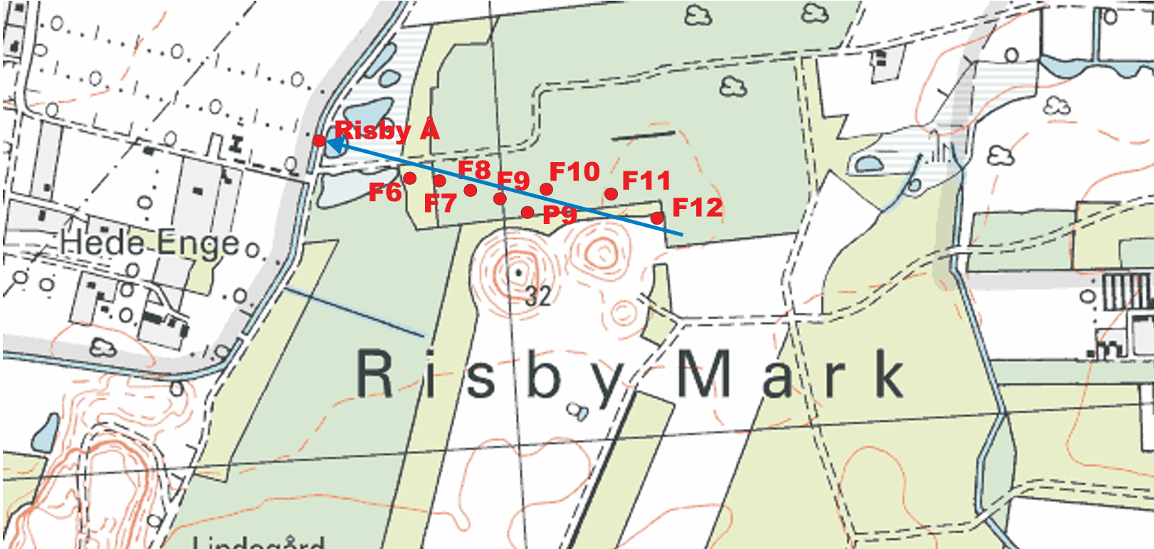
Figure 1: Map of the Vestskov landfill area. The three landfills can be seen as small elevations in the landscape. Immediately north of the landfills lies a transect of boreholes where the groundwater level has been measured.

Figure 2 shows a schematic sketch of the regional geology in the area. At the top, the area consists of about 2–4 meters of moraine sand, followed by about 18 meters of moraine clay. Limestone is encountered beneath this layer.

Figure 3 shows a cross section through the local area. This section is placed approximately along a streamline from F12 to Risby Stream. The figure shows the boreholes where the groundwater level (the hydraulic head, \(h\), sketched in the figure) has been measured. The figure also shows that there are two groundwater aquifers: an upper secondary groundwater aquifer (fine sand/silt) that is in contact with the nearby stream (Risby), as well as a lower primary groundwater aquifer in the limestone, which in the area is used for drinking water supply. The moraine clay separates the two groundwater aquifers.

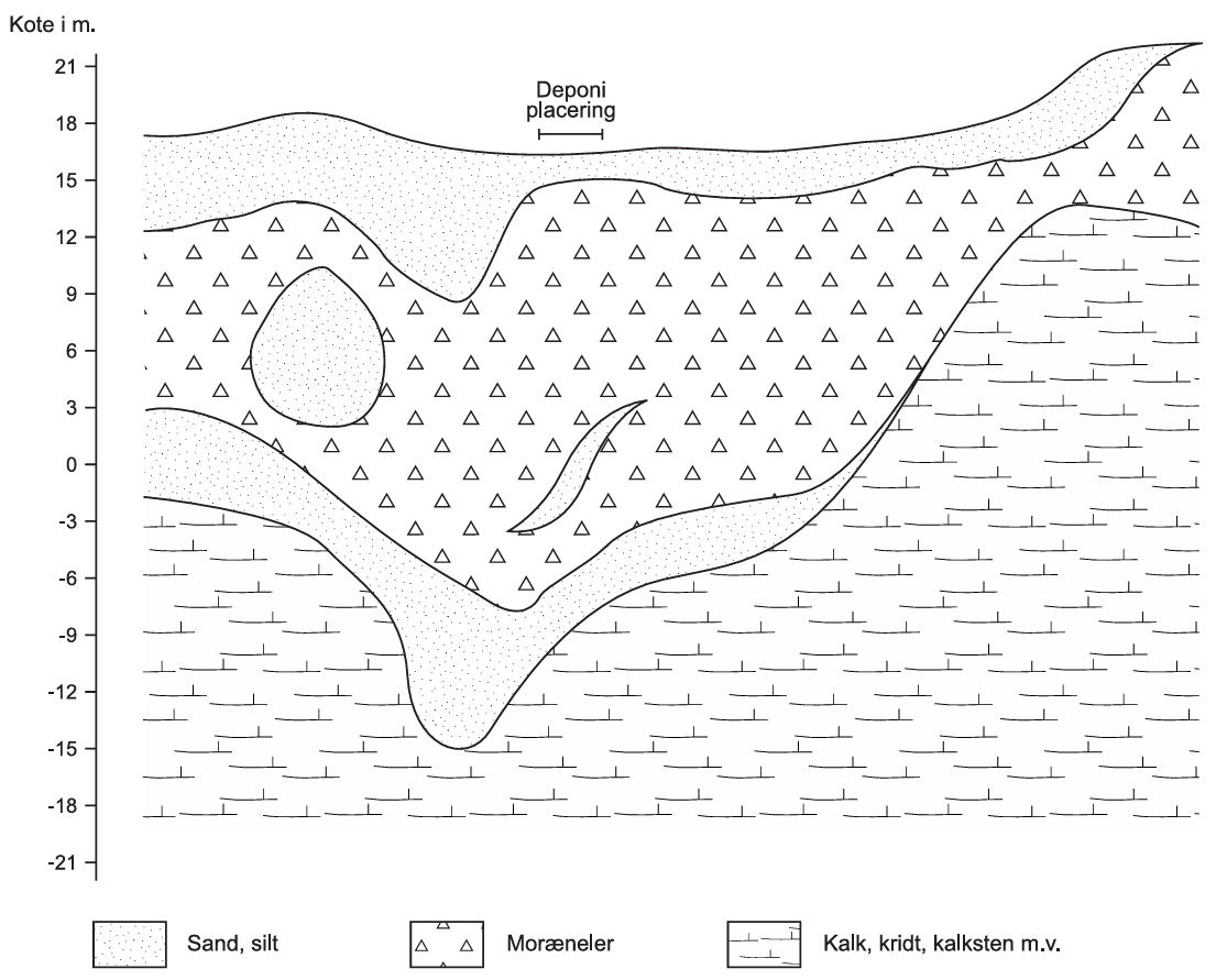
Figure 2: Regional geology in the area. The landfill area is shown in the figure. Danish terms in the figure translate as follows: deponi placering (landfill location), sand, silt (sand, silt), moræneler (glacial till), and kalk, kridt, sandsten, m.v. (limestone, chalk, sandstone, etc.).

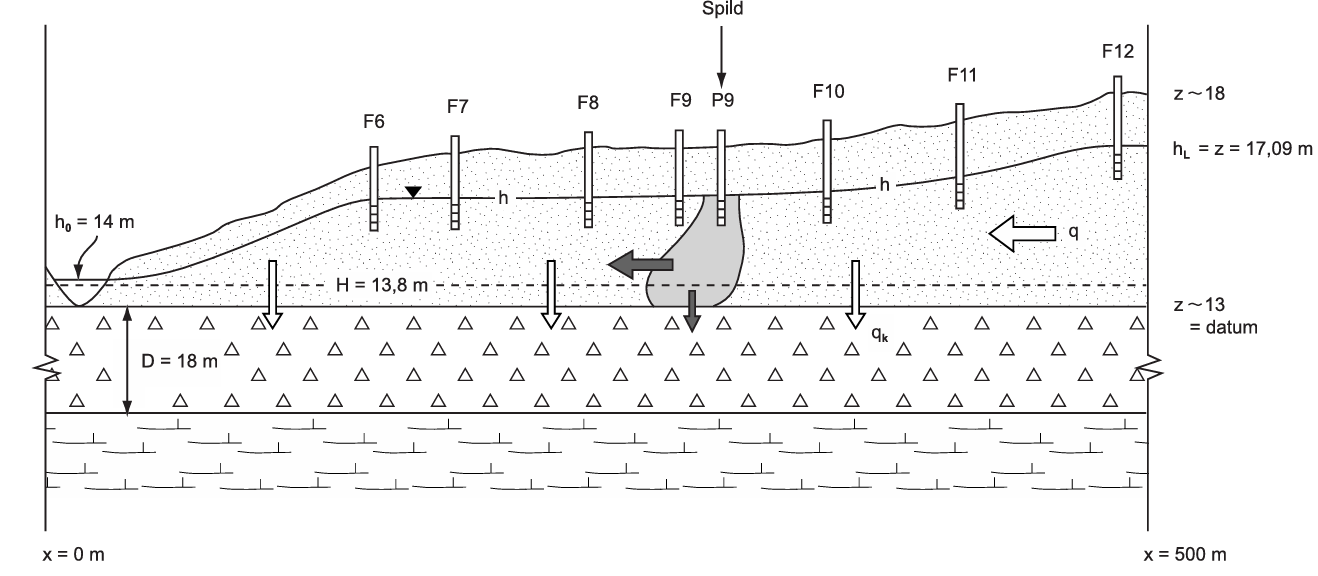
Figure 3: Transect with local geology, boreholes, and hydraulic heads in the upper and lower groundwater aquifer. Danish terms in the figure translate as follows: spild (spill) and datum (datum).

As sketched in Figure 3, there is a horizontal flow from east of the landfills down toward Risby Stream (\(q\) in Figure 3). This is because there is a head drop toward the stream. At the same time there is also a downward head gradient and flow (\(q_k\)) between the upper and lower aquifer, since the hydraulic head in the limestone everywhere can be assumed to be \(H=13.8\ \text{m}\), i.e. below the hydraulic head that is in the upper section, where \(h\) is about 14–17 m along the transect (the head is lower because water is pumped from the lower aquifer). The pollution in the area has occurred near borehole P9 (Figure 3). The pollution will therefore move horizontally toward the stream—and vertically toward the limestone aquifer.

Data

Data for the Vestskoven area are given in Tables 1 and 2 (below). The net infiltration to the groundwater is 200 mm/year (on average about 700 mm of rain falls per year, but about 500 mm drains and evaporates). The thickness of the moraine clay can be set to \(m=18\ \text{m}\) and the hydraulic head in the limestone is constant \(H=13.8\ \text{m}\).

A model for the head, \(h(x)\), in the upper groundwater aquifer is set up below for the transect shown in Figure 3. The transect is \(L=500\ \text{m}\) long and the boundary conditions are given by fixed hydraulic heads. At \(x=0\ \text{m}\) the head is \(h(0)=14.00\ \text{m}\) and at \(x=500\ \text{m}\) the head is the same as in F12, i.e. \(h(500)=17.09\ \text{m}\).

The two unknown parameters in the model are \(K_s\) and \(K_m\), which are the hydraulic conductivities for, respectively, the upper groundwater aquifer and the moraine clay that separates it from the lower groundwater aquifer in the limestone. In practice, hydraulic conductivities are determined experimentally.

On May 14, 1999, a number of hydraulic heads were measured, as shown in Table 2. The transect in Figure 3 is nearly parallel to east–west and Table 2 therefore shows the UTM (East) coordinates of the boreholes (UTM stands for Universal Transverse Mercator).

Table 1: Data from Vestskoven

Parameter	Value	Unit
Net infiltration, \(N\)	0.2	m/year
Datum, \(z_0\)	13	m
Thickness of moraine clay, \(m\)	18	m
Hydraulic head in limestone, \(H\)	13.8	m
Porosity in upper aquifer, \(\phi\)	0.21	–
Length of transect, \(L\)	500	m
Fixed head, \(h_0\)	17.09	m
Fixed head (the stream), \(h_L\)	14.00	m

Table 2: Observed hydraulic heads, \(h\), see Figure 3, and UTM-East coordinates

Borehole	UTM-East (m)	Head (m)
F12	333147	17.09
F11	333068	16.38
F10	333008	16.38
P9	332961	16.14
F9	332938	16.11
F8	332883	16.09
F7	332836	16.05
F6	332788	16.06
Risby Stream	332647	14.00

Exercise 3.1
(a) Make a plot in Sympy of the data points given in Table 2, for example of \(h(x)\) as a function of the distance to the stream, \(x\). The distance is computed from the UTM coordinates. What are the boundary conditions on the endpoint values for \(h\)?
(b) Consider what kind of \(n\)th-degree polynomial \(p_n(x)\) could immediately approximate the trend of the data points? Try, for example, to experiment with \(n=1,\dots,4\).

Physical model

In this section a physical model is set up to determine the head drop \(h\) as a function of the distance \(x\).

Flow of fluid in porous media is governed by Darcy’s law:

\[ Q=-K_s\cdot A\frac{\partial h}{\partial x}\tag{4.1} \]

where \(Q\) is the discharge (measured in m\(^3\)/s), \(h\) is hydraulic head (m), \(A\) is cross-sectional area (m\(^2\)), and \(K_s\) is the hydraulic conductivity of the groundwater aquifer (m/s). A \(K\)-value therefore characterizes how well “the geology conducts water”. Sand has a relatively high \(K\)-value (\(\sim 10^{-4}\)–\(10^{-3}\ \text{m/s}\)), while clay has a lower \(K\)-value (\(\sim 10^{-7}\)–\(10^{-6}\ \text{m/s}\)). It follows that a head gradient \((\partial h/\partial x\neq 0)\) is necessary to facilitate a flow, analogous to the fact that a potential difference is necessary to create a current in an electrical circuit.

In principle, the area \(A\) is a function of three variables \(A=A(x,y,z)\), i.e. it can vary in horizontal and vertical direction. In the following we will only look at a one-dimensional model. Here we set the area to \(A=(1\ \text{m}\cdot d)\), where \(d=h-z_0\) is the saturated thickness (m) in the sand, see Figure 3 (\(z_0\) is the datum, i.e. a reference point). In other words, everything is computed “per meter width”. The cross-sectional area therefore changes with distance depending on whether the groundwater level changes. With this, (4.1) is rewritten as

\[ Q=-K_s\cdot (h-z_0)\frac{dh}{dx}.\tag{4.2} \]

The discharge \(Q\) is therefore nonlinear with respect to \(h\) because there is a nonlinear term of the form \(h\frac{dh}{dx}\). In the following we use that the Darcy velocity is defined as flow per total area, i.e.

\[ q=\frac{Q}{A}=-K_s\frac{dh}{dx}.\tag{4.3} \]

A flow balance (total inflow = total outflow) can also be set up for the control volume in Figure 4, which expresses that no fluid accumulates in the control volume:

\[ -\frac{dQ}{dx}\,dx + N\,dx - q_k\,dx = 0.\tag{4.4} \]

Here \(N\) corresponds to the net infiltration on a yearly basis (i.e. precipitation minus actual evaporation; the part of the precipitation that reaches the groundwater). The quantity \(N\) can here be assumed constant corresponding to an average infiltration over a year, and \(q_k\) is the amount of water that is lost from the upper groundwater aquifer due to a gradient down toward the limestone. This water loss is not necessarily constant. The head in the limestone (\(H\), see Figure 3) can be considered constant, but since the upper head (\(h\)) varies, \(q_k\) will also vary, according to Darcy’s law written in the vertical direction:

\[ q_k=-K_m\cdot \frac{H-h}{m},\tag{4.5} \]

where \(K_m\) and \(m\) are, respectively, the hydraulic conductivity and the thickness of the moraine clay.

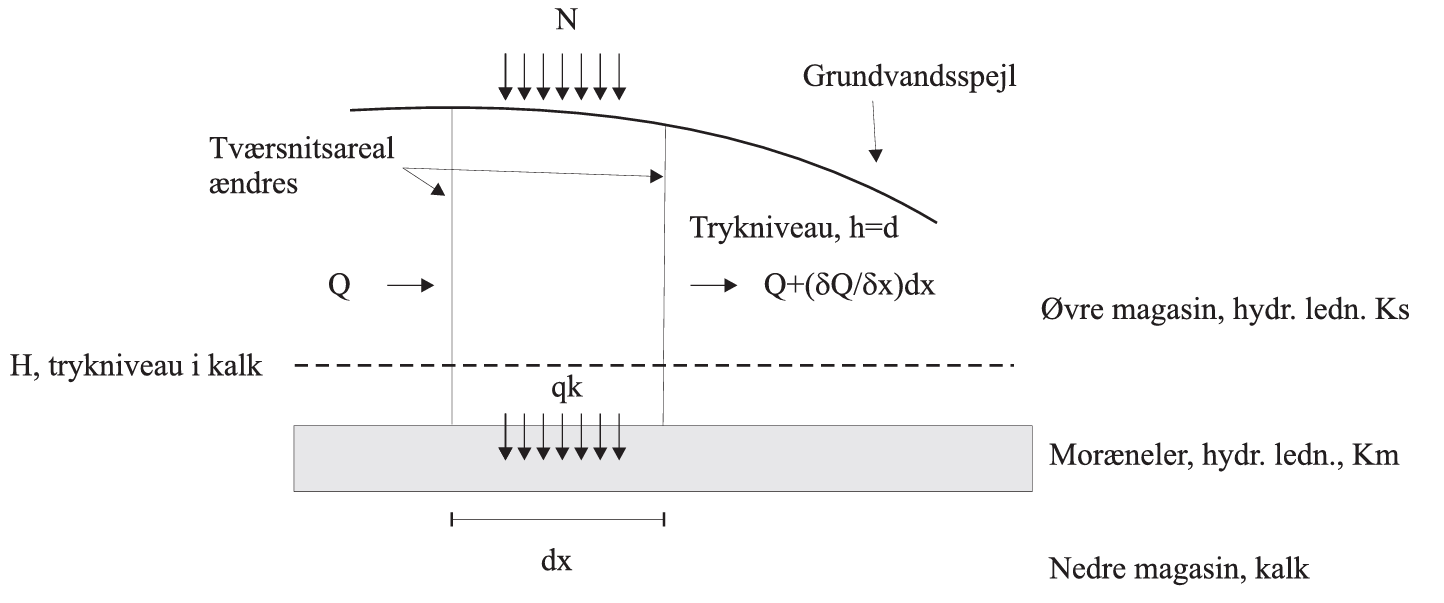
Figure 4: Control volume for setting up the flow balance. The cross section is shown from the opposite perspective compared to Figure 3. Danish terms in the figure translate as follows: Tværsnitsareal ændres (cross-sectional area changes), Grundvandsspejl (water table), Trykniveau i kalk (potentiometric surface in limestone), Øvre magasin, hydr. ledn. Ks (upper aquifer, hydraulic conductivity \(K_s\)), Moræneler, hydr. ledn. Km (glacial till, hydraulic conductivity \(K_m\)), and Nedre magasin, kalk (lower aquifer, limestone).

Solving differential equations

Exercise 5.1
(a) Derive, using the formulas from Section 4, that the head drop \(h(x)\) is determined by the differential equation

\[\begin{equation*} \frac{d^2\big((h-z_0)^2\big)}{dx^2}+\frac{2K_m}{K_s}\frac{H-h}{m}+\frac{2N}{K_s}=0.\tag{5.6} \end{equation*}\]

(b) What order differential equation is this? Why is it a nonlinear differential equation? Consider what other conditions \(h(x)\) must satisfy. This could, for example, be that \(h\) has given values at the endpoints of the interval where we seek to determine \(h\) (called boundary conditions).

Exercise 5.2
The differential equation (5.6) cannot be solved analytically. Even though one cannot solve (5.6) directly, one can say something about what a possible solution will look like.
(a) Define \(y(x)=h(x)-z_0\) and find an equation for \(y'(x)\) by applying equation (5.6). Concretely, one must show that \(y'(x)\) satisfies an equation of the form

\[\begin{equation*} y'(x)=\frac{1}{6y(x)}\sqrt{12Ay(x)^3-18By(x)^2+36C}.\tag{5.7} \end{equation*}\]

Can Sympy solve this equation for \(y(x)\)?
(Hint: Write (5.6) in the form \((y^2(x))''-Ay(x)+B=0\), multiply the left-hand side of (5.6) by \(y(x)y'(x)\) and integrate on both sides.)

Exercise 5.3
One way to approach (5.6) is to look at different limits, where the solution has a relatively simple form.
(a) First assume that the solution to the differential equation (5.6) is a constant function \(h(x)=h_K\) (even though this contradicts the boundary conditions). Derive an expression for \(h_K\) in terms of the given constants.
(b) Next assume that the solution is a linear function, \(h(x)=\alpha x+\beta\). Does there exist a solution \(h(x)\) to equation (5.6) with \(\alpha\neq 0\)?
(Hint: Insert the two different solutions into equation (5.6).)

We now know that the desired function \(h(x)\) cannot be a linear function, i.e. a straight line, but must have a more complicated form.

Exercise 5.4
(a) Set the hydraulic conductivities to \(K_m=5\cdot 10^{-8}\ \text{m/s}\) and \(K_s=3\cdot 10^{-6}\ \text{m/s}\) and determine from this an approximate value for \(h_K\) in Exercise 5.3 given the data in Table 1 (in the table, \(N\) is computed in m/year; it must be converted to m/s).
(b) Consider why the second term in the differential equation (5.6) must be small when \(h\approx H\). Then solve the differential equation (5.6) in the case where the second term (proportional to \(K_m/K_s\)) is ignored, i.e. find an exact solution in this case without using Sympy.
(Hint: If \((y(x)^2)''=\text{constant}\), then \(y^2(x)\) must be a quadratic polynomial.)

Exercise 5.5
One can simplify (5.6) by assuming that the cross-sectional area \(A\) in equation (4.1) is constant, i.e. that (4.1) is modified to

\[\begin{equation*} Q=-K_s\cdot d_0\frac{dh}{dx},\tag{5.8} \end{equation*}\]

where \(d_0\) is a constant, for example an average of \(h-z_0\) along the transect of boreholes.
(a) Use equations (4.4) and (4.5) to derive that the resulting differential equation corresponding to (5.6) in this case becomes

\[\begin{equation*} \frac{d^2(h-H)}{dx^2}-\frac{K_m}{d_0K_s m}(h-H)+\frac{N}{d_0K_s}=0,\tag{5.9} \end{equation*}\]

and that this is therefore a linear differential equation.
(b) What kind of differential equation is (5.9)? Solve (5.9) directly. (Hint: Solve the corresponding homogeneous equation first, then the inhomogeneous.)
Note that (5.6) is a differential equation for \(h-z_0\), while (5.9) is a differential equation for \(h-H\).

The model as a system of differential equations

Alternatively to solving a second-order differential equation (5.9), one can set up the model as a system of first-order equations.

The idea is to use the variables \(h\) and \(Q\) to write a system of first-order differential equations that is a model for the system, cf. equations (4.1) and (4.4). Note that these two equations express the horizontal flow and the vertical flow. We assume that \(A\) is constant equal to \(d_0\); thus (4.1) is replaced by (5.8).

Exercise 6.1
(a) Show that the system of differential equations (5.8) and (4.4) can be written in matrix form (you will also need equation (4.5)). Set up a set of equations of the form

\[\begin{equation*} y'(x)=Ay(x)+B,\tag{6.10} \end{equation*}\]

where \(y(x)=(h(x),Q(x))^T\), \(y'(x)=(h'(x),Q'(x))^T\), and \(A\) is a \(2\times 2\) matrix while \(B\) is a column vector.
(b) What kind of system of equations is this, and what does the complete solution look like according to the theory?

Exercise 6.2
Determine the solution to the corresponding homogeneous equation by diagonalizing \(A\), i.e. \(D=P^{-1}AP\), where \(D\) is a diagonal matrix and \(P\) is a square matrix determined by the eigenvectors of \(A\).
(a) Find the eigenvalues and eigenvectors for \(A\). First show that the eigenvalues are given by

\[\begin{equation*} \lambda_{\pm}=\pm\sqrt{\frac{K_m}{m d_0 K_s}}. \end{equation*}\]

(b) Then write the complete solution to (6.10) by determining a constant solution to \(y'(x)=0\). The complete solution depends on \(\lambda_{\pm}\) and on two unknown constants, which we call \(c_1\) and \(c_2\).

Exercise 6.3
We do not yet know the values of the hydraulic parameters from the given data. Therefore set \(K_m=5\cdot 10^{-8}\ \text{m/s}\) and \(K_s=3\cdot 10^{-6}\ \text{m/s}\) to start with. Furthermore, set \(d_0\) equal to the average of \(h-z_0\) along the boreholes.
(a) Insert these values for \(K_m\), \(K_s\) in the found solution and use Sympy to determine the two unknown constants \(c_1\), \(c_2\) using the boundary conditions for \(h(x)\).
(b) Plot \(h(x)\) and compare, if relevant, with the plot in Exercise 3.1.
(c) Optionally try to change \(K_m\) and \(K_s\) by up to \(\pm 10\%\) and see whether this gives a visibly better approximation to the data points.

Determination of the hydraulic parameters

Based on the data it should be possible to find values of the unknown hydraulic conductivities \(K_s\) and \(K_m\) by comparison with the model. When one needs to “calibrate” a given model, one can for example use a measure of the error between the model (the function \(h\)) and the measured data of the form

\[ \mathrm{ERR}=\left(\sum_{i=1}^{N}\left|h(x_i)-h_{\mathrm{meas}}(x_i)\right|^{p}\right)^{1/p}.\tag{7.11} \]

Here \(h_{\mathrm{meas}}(x_i)\) are the measured heads at the positions \(x_i\), \(i=1,\dots,N\) (\(N\) is the number of measurement points). The power \(p\) is chosen depending on what one wants to achieve; different choices of \(p\) correspond to different “sensitivities” to the model’s deviations from data. In the following we use \(p=2\).

Exercise 7.1
(a) Determine values of \(K_s\) and \(K_m\) that make the error ERR as small as possible for the data given in Table 2. For \(h(x)\) use the type of solution determined in Exercise 6.2, i.e. vary \(K_m\), \(K_s\) slightly away from the original values, and new values for \(c_1\) and \(c_2\) can then be determined using the boundary conditions. One can, for example, suffice with computing the error ERR at five points in the \((K_m,K_s)\)-plane: first with the values in Exercise 6.3. Then change \(K_m\) by \(\pm 10\%\) while keeping \(K_s\) fixed, and vice versa. Optionally one can investigate ERR as a function of \(K_m\) (keep \(K_s=3\cdot 10^{-6}\ \text{m/s}\)).

Exercise 7.2
(a) Use Sympy to determine the \(n\)th-degree polynomial \(p_n(x)\) that best matches the data. Try \(n=1,2,\dots,8\).
(b) Compute the error ERR for each of the eight polynomials in question (a).

Exercise 7.3
There exists a unique “Lagrange polynomial”, which is the polynomial of degree \(\le n\) that passes through \(n+1\) given points \((x_i,y_i)\).
(a) The data points in Table 2 consist of nine points. Determine the Lagrange polynomial that passes exactly through all points. Plot the Lagrange polynomial together with the data points, and compute ERR.

Transport of pollution

In the last part of the assignment one must investigate how fast pollution is transported by groundwater flow.

Darcy’s law (4.1) gives the flow per total cross-sectional area, \(A\). Since the area consists of sand grains and pore space (the area between sand grains), the pore water velocity is defined as

\[ v=\frac{q}{\phi},\tag{8.12} \]

where \(\phi\) is the porosity. The porosity is defined as the number of cubic meters of pore space per cubic meter of total volume and is therefore less than 1. The pore water velocity is therefore greater than the Darcy velocity, \(q\).

The average residence time in a piece of soil of a particle transported with the groundwater is found from velocity as a derivative:

\[ v=\frac{dx}{dt},\tag{8.13} \]

where \(x\) is the position of a particle after a given time \(t\). From this the residence time \(T\) of the particle over the interval \([x_1,x_2]\) can be computed as

\[ T=\int_{0}^{T}dt=\int_{x_2}^{x_1}\frac{1}{v}\,dx.\tag{8.14} \]

If the pore water velocity is constant, one gets in particular that the residence time in an interval of length \(l\) is

\[ T=\frac{l}{v}.\tag{8.15} \]

This gives the simple result that the residence time is length divided by speed. In the case where \(v\) is not constant with distance \(x\), the computation becomes a bit more complicated.

One can give an estimate of the residence time as follows, since approximately the pore water velocity between P9 and the stream can be computed via Darcy’s law as

\[ |v|=\frac{K_s}{\phi}\frac{\Delta h}{\Delta x}=\frac{3\cdot 10^{-6}}{0.21}\cdot\frac{16.14-14}{314} =9.7\cdot 10^{-8}\ \text{m/s}\approx 3.1\ \text{m/yr}.\tag{8.16} \]

Thus the residence time can be estimated as

\[ T=\frac{l}{|v|}=\frac{314}{3.1}\ \text{yr}=101\ \text{yr}.\tag{8.17} \]

With correct integration one will see that the time becomes something else, since the pore water velocity increases dramatically down toward the stream due to the smaller saturated thickness, just as it is almost zero in the middle of the transect. To make this more precise, one finds \(v(x)\) by differentiating the expression for \(h(x)\), cf. equation (8.16), where \(\Delta h/\Delta x\) is an approximation to the derivative. Then \(T\) is found by integration, cf. equation (8.14).

Exercise 8.1
(a) Find the pore water velocity \(v(x)\), and thereby the residence time \(T\) in the upper groundwater aquifer to the stream, if the particle is “released” at landfill 3, corresponding to borehole P9. For \(h(x)\) use the solution determined in Exercise 6.3.
(b) What happens to the residence time if the particle “begins its journey” at borehole F6? For \(h(x)\) use the solution determined in Exercise 6.3.

Exercise 8.2
(a) Consider whether these results are sensitive to the estimate of \(K_s\) and \(K_m\). What happens to the residence times if the two parameters are changed independently of each other by, for example, \(\pm 10\%\)?

Exercise 8.3
(a) What happens to the residence time if one uses the simple model from Exercise 7.2 (e.g. a 3rd-degree polynomial)? Is this model realistic?