import matplotlib
if not hasattr(matplotlib.RcParams, "_get"):
    matplotlib.RcParams._get = dict.get

Graphs and Networks

We are surrounded by networks everywhere: roads, railways, the internet, electronics, and friendships (both connections in real life and on social networks).

In mathematics, we can represent networks as graphs. A graph consists of nodes connected by edges. We draw them using circles (nodes) and lines (edges). An edge goes between two nodes. Two nodes are neighbors if there is an edge between them.

Example: Here is a graph with 5 nodes.

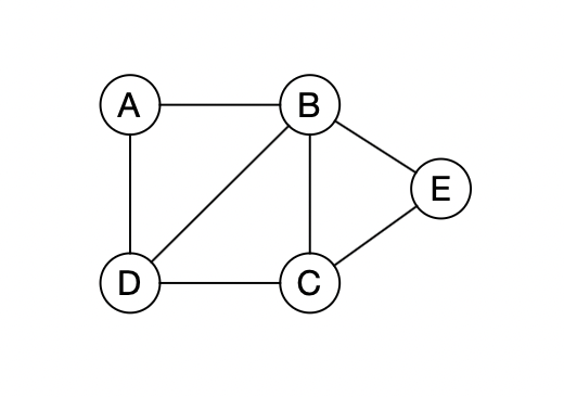
The position of the nodes and the length of edges in the drawing do not matter. We are only interested in how the nodes are connected to each other. The drawings below all represent the same graph.

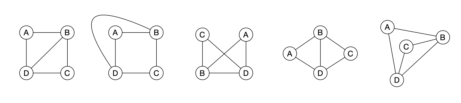
Which of the graphs below is different from the others?

The degree of a node is the number of neighbors. In the graph below, node \(B\) has degree \(4\). When we describe a graph without drawing it, we write the edges as pairs of nodes, e.g. \((A, B)\).

• How many nodes does the following graph have?

• How many edges?

• What is the degree of node \(A\)?

Setup

import networkx as nx
import matplotlib

if not hasattr(matplotlib.RcParams, "_get"):
    matplotlib.RcParams._get = dict.get

import matplotlib.pyplot as plt

Graphs in Python

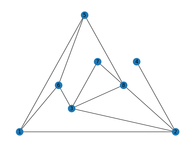
We can draw graphs in Python using the package networkx. Run the code below and answer:

• how many nodes are there in the graph \(G\)?

• how many edges?

• what is the maximum degree in the graph? (how many neighbors does the node with the most neighbors have?)

### Code that inserts the nodes here:

G = nx.Graph()
G.add_node(1)
G.add_node(2)
G.add_node(3)
G.add_node(4)
G.add_node(5)
G.add_node(6)
G.add_node(7)
G.add_node(8)

### ******************************
### Code that inserts the edges here:

G.add_edge(1,2)
G.add_edge(3,2)
G.add_edge(4,2)
G.add_edge(1,5)
G.add_edge(3,7)
G.add_edge(6,1)
G.add_edge(6,3)
G.add_edge(7,8)
G.add_edge(8,5)
G.add_edge(8,2)
G.add_edge(8,3)
G.add_edge(6,5)

### ******************************
### Draws the graph

nx.draw(G, pos=nx.planar_layout(G), with_labels=True)
plt.show(block=True)

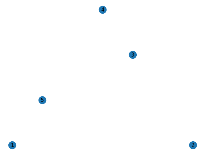
In the code cell below we build a new graph \(F\). The graph has 5 nodes numbered from 1 to 5. There are no edges in the graph.

F = nx.Graph()
F.add_node(1)
F.add_node(2)
F.add_node(3)
F.add_node(4)
F.add_node(5)
### **********
### Insert code that inserts the edges here:




### **********
### Draws the graph

nx.draw(F, pos=nx.planar_layout(F), with_labels=True)
plt.show(block=True)

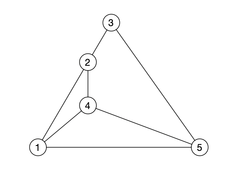
The function add_edge(i, j) creates an edge between node \(i\) and \(j\).

Insert edges using the add_edge function so that the graph has the same edges as the graph in the drawing below.

Neighbor command

We can use the following commands/functions in networkx to examine the graph:

• list(G.nodes): returns a list of all nodes in \(G\).

• list(G.neighbors(i)): returns a list of all neighbors of node \(i\).

• G.degree[i]: returns the degree of node \(i\).

We return to the graph \(G\) as defined earlier.

Run the following code. Modify it so that it prints the neighbor list for node \(4\) and the degree of node \(4\).

### ******************************
### Examine the graph G:

print('The graph has', len(list(G.nodes())), 'nodes')
print('Node list:', list(G.nodes()))
print('Neighbors of node 3:', list(G.neighbors(3)))
print('Node 8 has degree:', G.degree(8))

### ******************************
### Draws the graph

nx.draw(G, pos=nx.planar_layout(G), with_labels=True)
plt.show(block=True)

The graph has 8 nodes
Node list: [1, 2, 3, 4, 5, 6, 7, 8]
Neighbors of node 3: [2, 7, 6, 8]
Node 8 has degree: 4

Add code below that loops through all nodes in the graph \(G\) and computes and prints the sum of the degrees.

# Find the sum of degrees:

Add code below that loops through all nodes in the graph \(G\) and finds the maximum degree in the graph.

# Find the maximum degree:

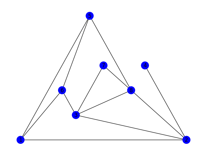
Colors

We can change the colors of nodes and edges individually by writing:

G.edges[i, j]['color'] = 'red',

G.nodes[i]['color'] = 'green'.

Add code to the graph below that

• colors all neighbors of node \(3\) green.

• colors all edges that have an endpoint in node \(3\) red.

### Color the graph:
# Add colors to edges and nodes here



### Draws the graph

e_colors = [c for u,v,c in G.edges.data('color', default='black')]
n_colors = [c for u, c in G.nodes.data('color', default='blue')]

nx.draw(G, pos=nx.planar_layout(G), edge_color = e_colors, node_color = n_colors, with_labels=True)
plt.show(block=True)

Shortest paths

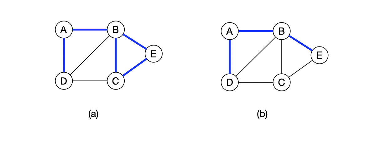
A walk of length \(k\) in a graph is a sequence of \(k\) edges

\[ (v_0,v_1),(v_1,v_2),(v_2,v_3),\dots,(v_{k-1},v_k). \]

However, a walk is most often given simply as the sequence of nodes it goes through: \(v_0,v_1,v_2,\dots,v_k\). A path is a walk where all nodes are different.

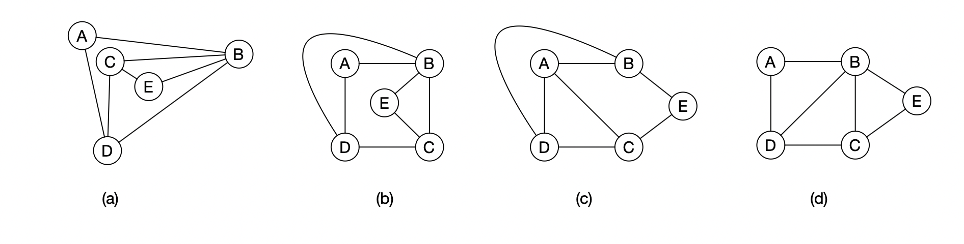
Example: Figure \((a)\) shows the walk \(B\), \(C\), \(E\), \(B\), \(A\), \(D\). Figure \((b)\) shows the path \(D\), \(A\), \(B\), \(E\).

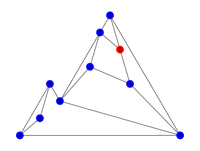
Run the code below and view the graph.

Add code that colors the edges of a path from node \(0\) to \(4\) (there are many different paths from \(0\) to \(4\); you just need to color one of them).

G = nx.Graph()
G.add_node(0)
G.add_node(1)
G.add_node(2)
G.add_node(3)
G.add_node(4)
G.add_node(5)
G.add_node(6)
G.add_node(7)
G.add_node(8)
G.add_node(9)

### **********
### Edges

G.add_edge(0,1)
G.add_edge(1,3)
G.add_edge(3,6)
G.add_edge(4,6)
G.add_edge(0,8)
G.add_edge(7,1)
G.add_edge(2,4)
G.add_edge(7,6)
G.add_edge(2,3)
G.add_edge(5,3)
G.add_edge(8,5)
G.add_edge(6,8)
G.add_edge(0,5)
G.add_edge(7,8)
G.add_edge(2,9)
G.add_edge(4,9)

### **********
### Insert code that colors edges on a path from 0 to 4 here:


### **********
### Draws the graph

colors = [c for u,v,c in G.edges.data('color', default='black')]
n_colors = [c for u, c in G.nodes.data('color', default='blue')]

nx.draw(G, pos=nx.planar_layout(G), edge_color = colors, node_color = n_colors, with_labels=True)
plt.show(block=True)

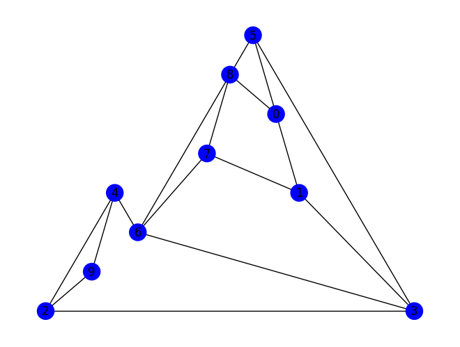
How long is the shortest path from node \(0\) to node \(4\)? How long is the longest path from node \(0\) to node \(4\) (remember that a path may only pass through a node once)?

Shortest path

In the following part we go through an algorithm to find a shortest path in a graph from a node \(v\) to all other nodes in a graph. We will develop it step by step until we have the final algorithm.

We say that a node \(u\) has distance \(d\) to node \(v\) if the length of the shortest path between \(u\) and \(v\) is \(d\). The algorithm should create a distance list where there is a \(d\) in position \(i\) if the distance between node \(0\) and node \(i\) is \(d\).

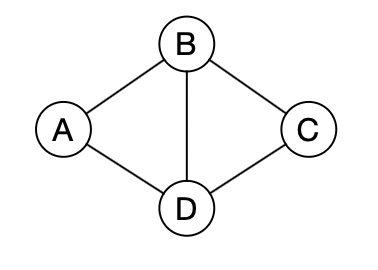
Example. The distance list for the graph below is \([0, 2, 3, 1, 1, 2]\).

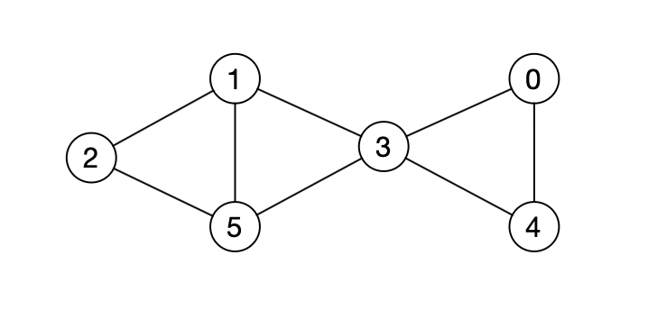
The overall idea of the algorithm is to first find all nodes that have distance \(1\) from node \(0\), then all nodes with distance \(2\), etc.

Distance 1

We will now make the first part of the algorithm, which finds all nodes with distance \(1\) to our start node \(0\). Look at the code below. In the distance list distance_list there is one entry for each node. To start with, there is \(-1\) in all positions.

#############################################
### Creates and updates distance list

distance_list = [-1]*10    # Creates an "empty" distance_list of length 10.

#### Insert code here 



#### Prints the distance list
print("distance_list:\n", distance_list)

##################
### Draws the graph

nx.draw(G, pos=nx.planar_layout(G), with_labels=True)
plt.show(block=True)

distance_list:
 [-1, -1, -1, -1, -1, -1, -1, -1, -1, -1]

Write code above that automatically modifies the distance list so that it contains the correct distance for all nodes that have distance at most \(1\) to node \(0\). For all other nodes there should still be \(-1\).

Hint: Use a for-loop and G.neighbors(i).

Distance 2

We will now find all nodes with distance \(2\) from node \(0\). All nodes that have distance \(2\) from node \(0\) must be a neighbor of a node that has distance \(1\) from node \(0\).

Why?

We will now modify the distance list from before so that it contains the correct distance for all nodes that have distance at most \(2\) to node \(0\). For all other nodes there should still be \(-1\).

Add code below that automatically modifies the distance list from before.

Remember: There should not be a \(2\) where there was previously a \(0\) or \(1\) in the distance list.

####################################
##### Write code that modifies the distance list

for i in range(10):
    if distance_list[i] == 1:
        #### Add code here ######

        ####

  Cell In[10], line 8
    ####
        ^
SyntaxError: incomplete input

All distances

We can find the distance from node \(0\) to all nodes in the graph by continuing in the same way. That is, round by round we find all the nodes that have distance one more than in the previous round.

Explain why the longest distance from one node to another can be at most the number of nodes in the graph minus one.

The code below contains a function BFS(v,G) that finds distances to all nodes in the graph \(G\) from the node \(v\).

Explain what the code does.

def BFS(v, G):
    '''
    Distance list from node v in graph G.
    '''
    N = len(G.nodes()) # number of nodes in G

    distance_list = [-1]*N # Creates an "empty" distance_list of length N.  

    distance_list[v] = 0 # The distance from v to itself is 0.

    # BFS algorithm
    for d in range(1,N):
        for i in range(N):
            if distance_list[i] == d-1:
                for j in G.neighbors(i):
                    if distance_list[j] == -1:
                        distance_list[j] = d

    return distance_list

The code cell below shows the distance list to node \(0\).

print('Distance list for node 0:\n', BFS(0, G))

Distance list for node 0:
 [0, 1, 3, 2, 3, 1, 2, 2, 1, 4]

BFS stands for breadth-first search and is a well-known algorithm for finding shortest paths in a graph.

Try calling the BFS function with a node other than node \(0\) and check that it finds the correct distances.

The code below is the same as above, but now there is a list of colors color_list.

Add code so that all nodes with distance \(d\) to node \(v\) get the color color_list[d].

def bfs_colors(v, G):
    '''
    Distance list from node v in graph G. Colors nodes by distance from v.
    '''
    # list of colors
    color_list = ['red', 'green', 'blue', 'cyan', 'orange', 'purple', 'brown', 'gray',' olive']


    N = len(G.nodes()) # number of nodes in G

    distance_list = [-1]*N   # Creates an "empty" distance_list of length N.

    # The distance from v to itself is 0
    distance_list[v] = 0
    G.nodes[v]['color'] = color_list[0]

    # BFS algorithm
    for d in range(1,N):
        for i in range(N):
            if distance_list[i] == d-1:
                for j in G.neighbors(i):
                    if distance_list[j] == -1:
                        distance_list[j] = d
                        # Insert code for coloring

                        ####

    return distance_list

######################
### Colors the graph with bfs_colors
bfs_colors(0, G)

######################
### Draws the graph
e_colors = [c for u,v,c in G.edges.data('color', default='black')]
n_colors = [c for u, c in G.nodes.data('color', default='blue')]

nx.draw(G, pos=nx.planar_layout(G), edge_color = e_colors, node_color = n_colors, with_labels=True)
plt.show(block=True)

Maze task

The figure below shows a maze. It can be modeled as a graph by creating a node for each cell and an edge between two cells if you can walk between them.

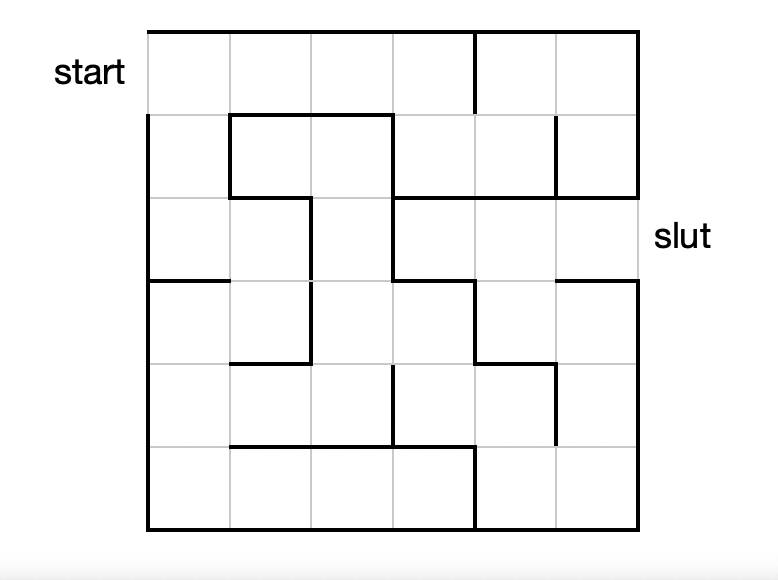
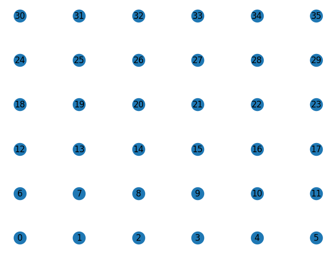
In the code cell below we create a graph with a number of nodes corresponding to all the cells, but there are no edges.

Run the code to see the nodes.

Add the edges and find the length of the shortest path from start to finish.

maze = nx.Graph()

########### Nodes ########
for i in range(36):
    maze.add_node(i)

########### Insert edges here ########


########### Draws the graph ###########
pos = {}

for i in range(6):
    for j in range(6):
        pos[i + j*6] = (i,j)
print(pos)

nx.draw(maze, pos, with_labels=True)
plt.show(block=True)

{0: (0, 0), 6: (0, 1), 12: (0, 2), 18: (0, 3), 24: (0, 4), 30: (0, 5), 1: (1, 0), 7: (1, 1), 13: (1, 2), 19: (1, 3), 25: (1, 4), 31: (1, 5), 2: (2, 0), 8: (2, 1), 14: (2, 2), 20: (2, 3), 26: (2, 4), 32: (2, 5), 3: (3, 0), 9: (3, 1), 15: (3, 2), 21: (3, 3), 27: (3, 4), 33: (3, 5), 4: (4, 0), 10: (4, 1), 16: (4, 2), 22: (4, 3), 28: (4, 4), 34: (4, 5), 5: (5, 0), 11: (5, 1), 17: (5, 2), 23: (5, 3), 29: (5, 4), 35: (5, 5)}

Connected components

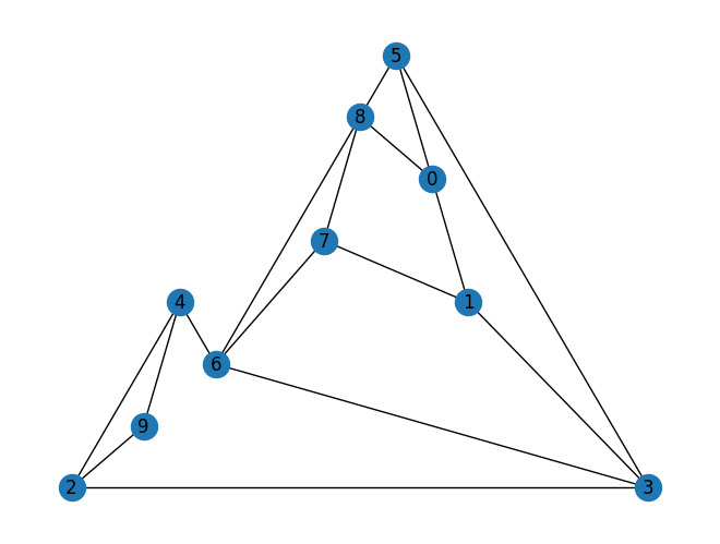
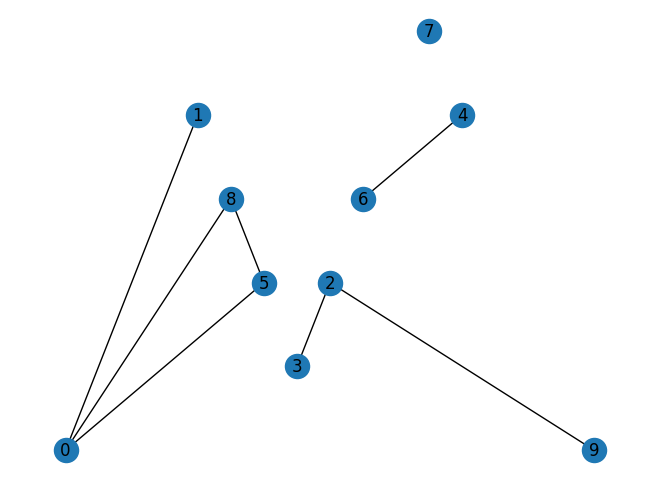
Until now we have only looked at what we call connected graphs (there exists at least one path between all pairs of nodes). The graph below is not connected.

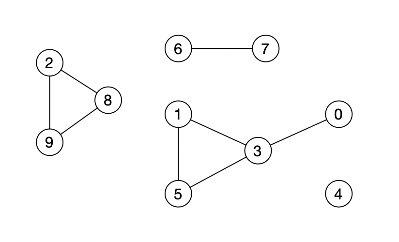
We say that two nodes are in the same connected component if there is a path between them.
The graph above has \(4\) connected components: \(\{2,8,9\}, \{6,7\}, \{0,1,3,5\}, \{4\}\).

In the following code cell a new graph \(H\) is defined.

Run the cell. Is \(H\) connected?

H = nx.Graph()
H.add_node(0)
H.add_node(1)
H.add_node(2)
H.add_node(3)
H.add_node(4)
H.add_node(5)
H.add_node(6)
H.add_node(7)
H.add_node(8)
H.add_node(9)
#############################################
### Edges

H.add_edge(0,1)
H.add_edge(4,6)
H.add_edge(0,8)
H.add_edge(2,3)
H.add_edge(8,5)
H.add_edge(0,5)
H.add_edge(2,9)

##################
### Draws the graph
nx.draw(H, pos=nx.planar_layout(H), with_labels=True)
plt.show(block=True)

We can use BFS to find connected components in a graph.

• Use the BFS function to create a distance list for node \(0\).

• Then use the distance list to create and print a list where there is a \(1\) for all nodes that are in the same connected component as node \(0\) and \(-1\) for all other nodes.

#############################################
### Add code that creates the distance list from node 0 in graph H



#######################################
## Add code that prints a list where there is 1 for
## all nodes that are in the same
## connected component as node 0.

Task: The Sun Islands

Adam is going on vacation to the archipelago paradise The Sun Islands. There are \(12\) islands and you can travel between islands by ferry or by using bridges. Adam does not like sailing, so he would like to know how many islands he can visit without sailing if he starts on island number \(5\) (the islanders strongly disagreed about who should be allowed to be called The Sun Island, so instead of giving the islands names they numbered them from \(0\) to \(11\)).

There are ferries between the following pairs of islands:

\[ (0,7), (0,1), (1,10), (2,6), (10,11). \]

There are bridges between the following pairs of islands:

\[ (4,6), (0,3), (2,5), (1,8), (1,3), (2,9), (3,8), (5,9), (5,10), (6,7), (9,11). \]

How many islands can Adam visit without sailing?

Explain how the problem can be modeled as a graph and draw the graph.

Write code in the box below that solves the problem.

G = nx.Graph()
########## Insert nodes here ######
# (add nodes)

######### Insert edges here ######
# (add edges)

####### Insert code that finds out how many islands Adam can visit ########
# (your code)

####### Remember that you can use the BFS function ########
# (call BFS)

######## Draws the graph ##################
nx.draw(G, pos=nx.planar_layout(G), with_labels=True)
plt.show(block=True)

All connected components

We can also use BFS to find all connected components in a graph. In the following, we want to create a component list for the graph. In the component list, the same number should appear for 2 nodes if they are in the same connected component.

Example: The list \([1, 1, 2, 1, 3, 1, 4, 4, 2, 2]\) is a component list for the graph below.

To find all connected components, we first use BFS to find all nodes that are in the same connected component as node \(0\). We write \(1\) for them in the component list. Then we find a node that is not in the same connected component as node \(0\) and use BFS to find all the nodes in its connected component. We write \(2\) for them in the component list. We continue like this until all nodes have received a number.

We return to the graph \(H\) as defined earlier. The following code cell redraws the graph.

### Draws the graph
nx.draw(H, pos=nx.planar_layout(H), with_labels=True)
plt.show(block=True)

Insert code in the following code cell so that component_list contains all connected components for the graph \(H\).

N = len(H.nodes()) # number of nodes in H

### Creates the component list with -1 in all positions
component_list = [-1]*N

### For-loop to fill the component list
for i in range(N):
    if component_list[i] == -1:
        # Distance list from node i
        distance_list = BFS(i,H)

        ## Write code here that updates the component_list


print("component_list:\n", component_list)

component_list:
 [-1, -1, -1, -1, -1, -1, -1, -1, -1, -1]

Task: Back to The Sun Islands

We return to the island group The Sun Islands. Adam still prefers not to sail and therefore wants to find out which island he should start on so that he can visit as many islands as possible without a ferry trip.

Insert code in the cell below that constructs a graph and uses it to solve the problem.

G = nx.Graph()
########## Insert nodes here ######
# (add nodes)

######### Insert edges here ######
# (add edges)

######### Insert code that computes which island Adam should start on ######
# (your code)

### Draws the graph
nx.draw(G, pos=nx.planar_layout(G), with_labels=True)
plt.show(block=True)

However, Adam would prefer to be able to visit all the islands, and he therefore accepts that he has to sail.

How few times can he get away with sailing in order to visit all the islands? Use the code cell below to solve the problem.

G = nx.Graph()
########## Insert nodes here ######
# (add nodes)

######### Insert edges here ######
# (add edges)

######### Insert code that finds the smallest number of times Adam must sail ######
# (your code)

### Draws the graph
nx.draw(G, pos=nx.planar_layout(G), with_labels=True)
plt.show(block=True)